Module 9: READING FROM AND WRITING TO FILES

Lesson 9.2 – Writing to Files

Lesson Objectives

After reading this lesson, you should be able to:

write numeric data to text files using MATLAB,
write numeric data to Excel files using MATLAB,
write non-numeric data to text files using MATLAB,
write non-numeric data to Excel files using MATLAB,
apply the concept of a delimiter when writing data.

How can I write numeric data to files with MATLAB?

Many of the concepts we learned when reading from files in Lesson 9.1 using dlmread() are also applicable when we use dlmwrite() for writing to a file. dlmwrite() is not the only method for writing to files, but it is one of the most straightforward. Similarly to dlmread(), dlmwrite() can only handle numeric data. Also, although we focus on writing to text files here, dlmwrite() is also compatible with the common .csv (comma separated values) file format.

Example 1

Write the numeric-only data given in matrix [A] to a file called ‘numeric_data.txt’ using dlmwrite().

\[\left\lbrack \text{A} \right\rbrack = \begin{bmatrix} \text{10} & \text{5} & \text{11} \\ \text{89} & \text{0.1} & \text{4} \\ \text{16} & \text{46} & \text{9} \\ \end{bmatrix}\]

Solution

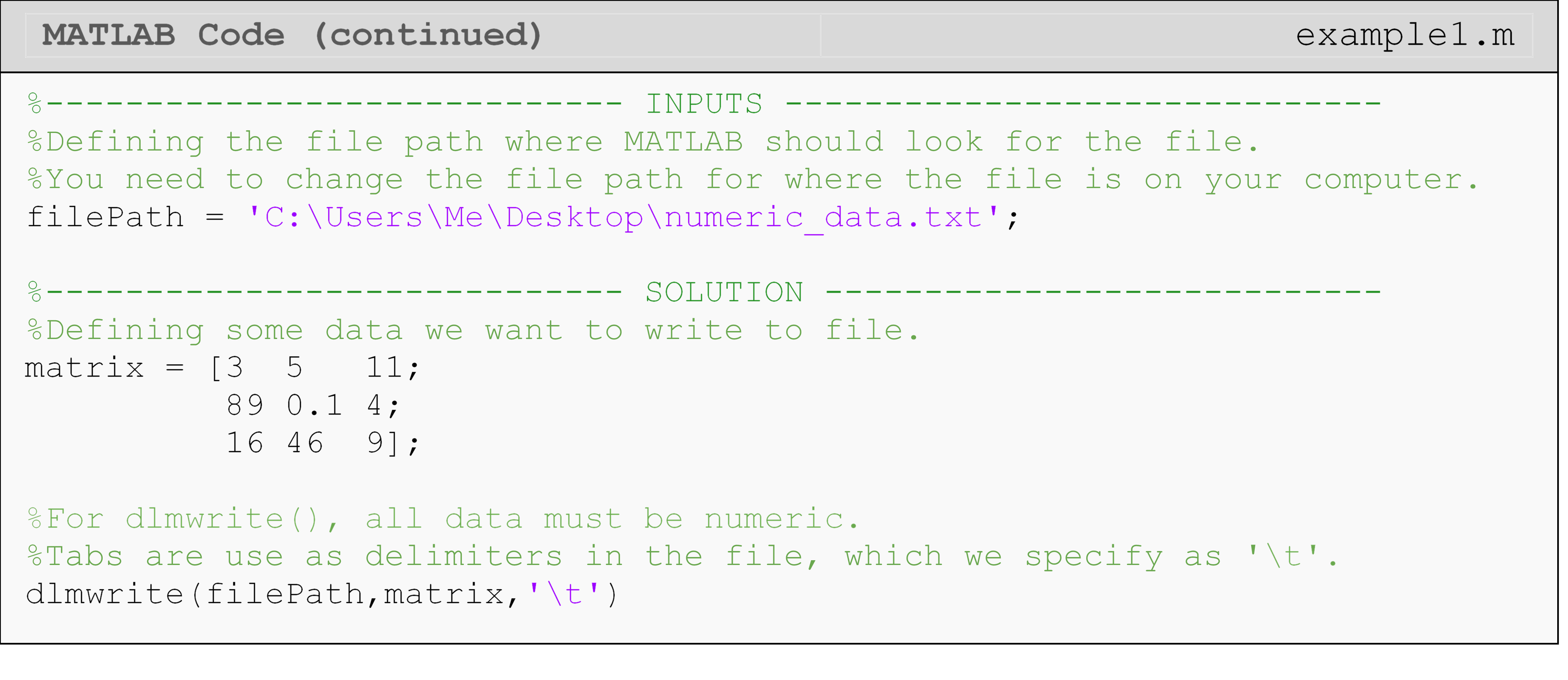
Note, the generated file shown in Figure 1 is opened in WordPad. This is because NotePad does not recognize end-of-line characters and would not properly display the matrix without adding some additional parameters to dlmwrite(). This is a minor detail and not something to be concerned about.

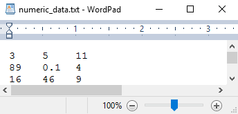
Figure 1: The opened file that contains the data we wrote to it in Example 1. You can use WordPad or equivalent program to create/edit .txt files.

We do not need to tell dlmwrite() to create a file as it will do so automatically if the file does not already exist. If a file does exist, it will overwrite the data contained in the file unless the append parameter is used (see documentation). Likewise, it will open and close the file automatically.

How can I write non-numeric data to files with MATLAB?

To write mixed data types (for example, numbers and strings), we need a way to store the data we want to write, and we need a write (or “print”) function that can handle both numeric and nonnumeric data. Previously, we used fprintf() to print messages to the Command Window, but now we will use it to write data to a text (.txt) file. The syntax and function of fprintf() are almost exactly the same in this application except we now need to give it the fileID, which is a unique identifier for that file (in case multiple files are open), to write to as seen in Example 2. You can see the lesson on Reading from Files (Lesson 9.2) for details on why we need fopen() and fclose().

Example 2

Write non-numeric (strings) and numeric (numbers) data to a file named ‘nonnumeric_data.txt’. Write the data given in the matrix [A] to the file. The first column of the file should be a label for each row in the form “first row”, “second row”, etc. For example, the first row written to the text file should read “first row 10 5 11”.

\[\left\lbrack \text{A} \right\rbrack = \begin{bmatrix} \text{10} & \text{5} & \text{11} \\ \text{89} & \text{0.1} & \text{4} \\ \text{16} & \text{46} & \text{9} \\ \end{bmatrix}\]

Solution

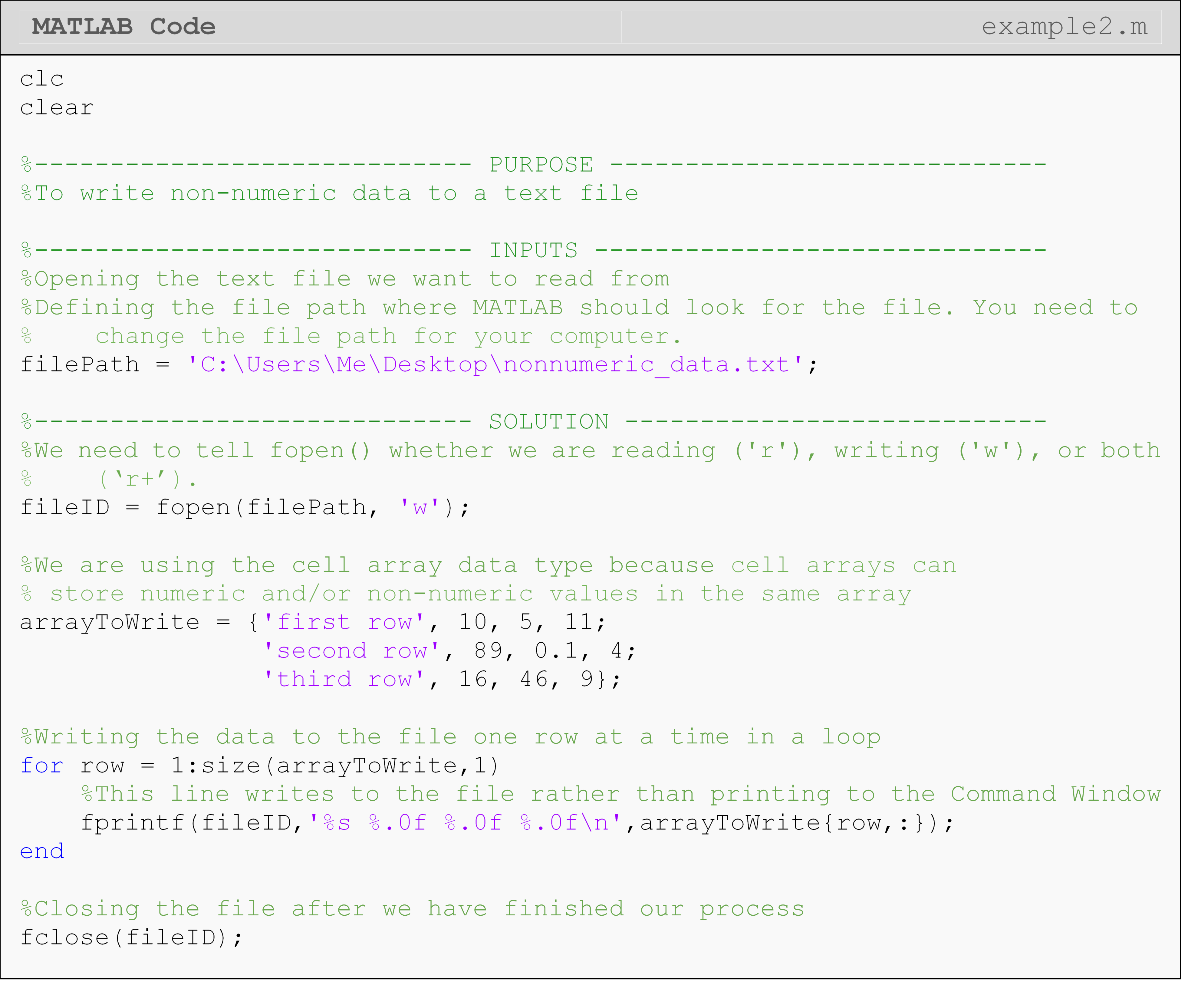
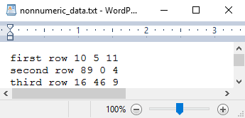
Figure 2: The opened file that contains the data we wrote to it in Example 2.

You can use Notepad, WordPad, or equivalent program to create/edit .txt files. As you can see in the opened text file in Figure 2, each row of the data is written to a line in the text file. In Example 2, all the strings are in the first column, so we knew which columns would contain only strings and which only numbers.

In some cases, you may want to write data in a more readable format such as to an Excel spreadsheet using xlswrite() or to a table format using writetable(). Example 3 shows how to write data to an Excel file using the xlswrite() function. As mentioned in Lesson 9.1, you can review MATLAB documentation on “Supported File Formats for Import and Export” for a quick reference on all the different options.

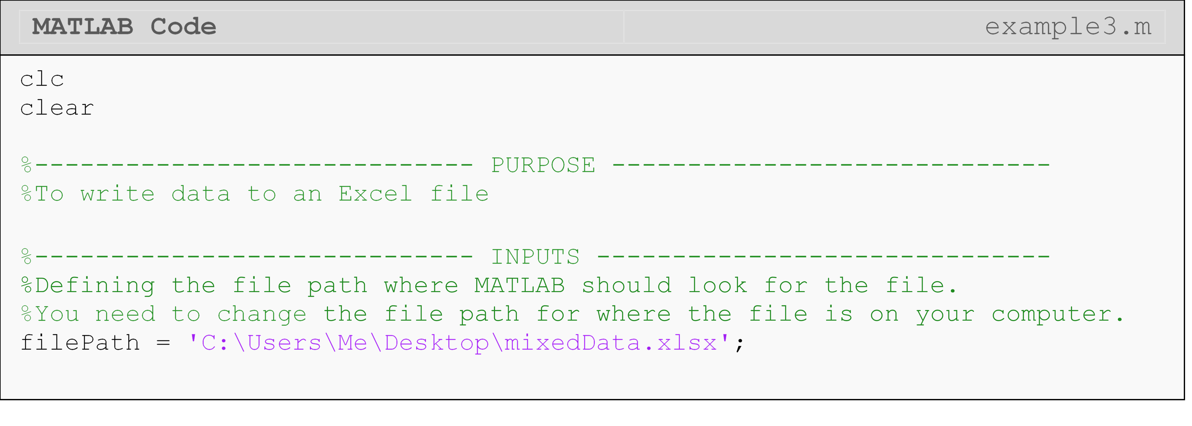
Example 3

Write non-numeric (strings) and numeric (numbers) data to an Excel file named ‘mixedData.xlsx’. Write the data given in matrix [A] to the file. The first column of the file should be a label for each row in the form “first row”, “second row”, etc. For example, the first row written to the text file should read “first row 10 5 11”.

\[\left\lbrack \text{A} \right\rbrack = \begin{bmatrix} \text{10} & \text{5} & \text{11} \\ \text{89} & \text{0.1} & \text{4} \\ \text{16} & \text{46} & \text{9} \\ \end{bmatrix}\]

Solution

As seen in Figure 3, the rows and columns of the cell array in MATLAB are written as rows and columns in the Excel spreadsheet.

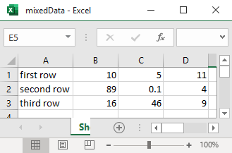
Figure 3: The opened Excel file that contains the data we wrote to it in Example 3.

Lesson Summary of New Syntax and Programming Tools

Task	Syntax	Usage
Write to an Excel file	xlswrite()	xlswrite(filePath,array)
Write to a text file	dlmwrite()	dlmwrite(filePath,array)

Multiple Choice Quiz

(1). The dlmwrite() function can write data containing

(a) numeric-only

(b) character-only

(d) None of the above

(2). Appending data to a file means MATLAB will

(a) Erase all the data in the file and then write the new data

(b) Add the new data to the beginning of the file and leave existing data intact

(d) do nothing because MATLAB cannot append data

(3). To open a file for writing, the correct choice is

(a) fopen(filePath)

(b) fopen(filePath,'r')

(d) fopen(filePath,'o')

(4). To write a line to an external text file, the most appropriate function is

(a) fgetl()

(b) fopen()

(d) fprintf()

(5). Complete the code to output the variable, a, to the text file, fo.

(a) fprintf(fwrite,'The number is %g',a)

(b) fprintf('The number is %g',a)

(d) disp(fwrite,a)

Problem Set

(1). Use the rand() function to generate some “sensor readings”. Assume our pseudo-sensor reports location in 3D space, and create “readings” for each axis (x, y, z). Pick a range that makes sense to you and generate at least 100 numbers for each variable. Write each of these variables to a text file (.txt) and an Excel file (.xlsx). The first column in the file should be the time associated with the sensor reading. Assume time starts at 0 and readings are taken every 0.01 seconds. The first row in the file should have a label for each row: namely, “time”, “x”, “y”, “z”.

(2). Create the text file shown below in Figure A, which contains polar coordinates (r, \(\theta\)). Read the file into MATLAB, convert the polar coordinates to Cartesian coordinates (x, y), and write the Cartesian coordinates to an Excel file called ‘cartCoords.xlsx’. The first row should be the labels for each column (“x” and “y”).

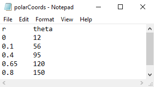
Figure A: A text file containing polar coordinate data.

(3). The Young’s modulus was calculated from discrete data in Lesson 9.1 Exercise 3. Append the text file that was used in Lesson 9.1 Exercise 3 with the calculated Young’s modulus and a description (e.g., “The Young’s modulus is …”) with appropriate units. Be sure not to overwrite the original data contained in the text file.

(4). Write matrix [D], given below, to a text file. In the same file, on separate lines, write:

“The size of the matrix is …”
“The norm of the matrix is …”
“The trace of the matrix is …”

\[\left\lbrack \text{D} \right\rbrack = \begin{bmatrix} \text{16} & \text{2} & \text{3} \\ \text{5} & \text{11} & \text{10} \\ \text{9} & \text{7} & \text{6} \\ \end{bmatrix}\]

Hint: To avoid hardcoding, you use loops to write the matrix such that your solution will work for a file containing any number of rows. Assume that [D] will be of size \(\text{3} \times \text{m}\) (i.e., it will always have three columns).

(5). Using the solution from Lesson 9.1 Exercise 1, append the sum of each row to the same m-file (‘exercise1.txt’) in the form “The sum of row X is …”. Use loops such that your solution will work for a file containing any number of rows.