Module 8: Loops

Lesson 8.6 – Applied Loops

Learning Objectives

After reading this lesson, you should be able to:

sort matrices and vectors,
search matrices and vectors,
sum matrices and vectors,
plot inside of a loop (repeated plotting),
use common programming tricks for loops.

Why is this lesson important?

There are a few common tasks using loops that are essential to understand how to implement them manually. We will cover how to sort, sum, and search in a vector (and a few other things). These have corresponding MATLAB functions that do not require you to do any of this, but knowing how to do these things not only gives you more practice with the programming concepts we have learned, but it also enables you to implement parts of these strategies in other solutions you write (that are not available as predefined functions).

Also, note that the content of this lesson is mostly contained in the example programs, so it is imperative to have a good understanding of these.

How can I sort an array?

Although there are predefined functions in MATLAB like sort(), it is useful to understand how to sort a vector manually. Bubble sort compares two adjacent elements and determines through a condition whether they need to be swapped to have a sorted vector.

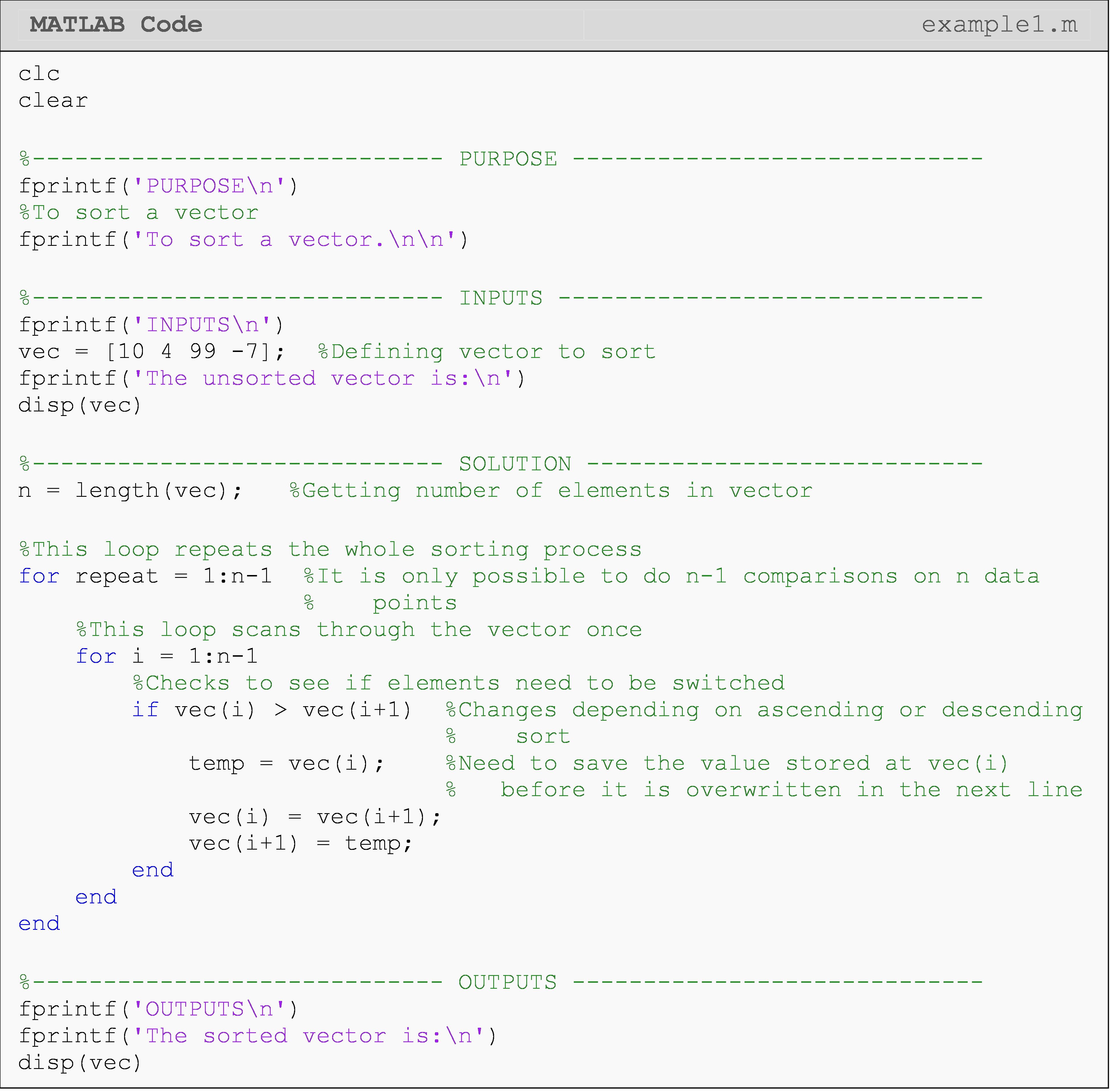
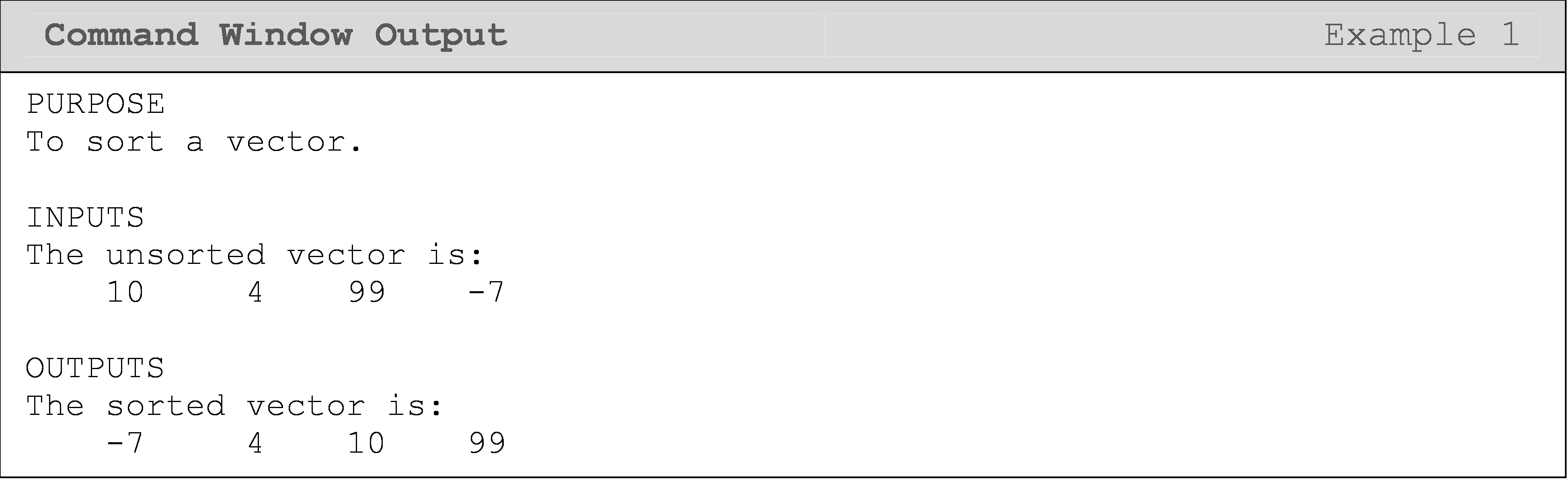
Example 1

Sort any given vector of numbers from smallest to largest. Test the program with the vector

[v] = [10 4 99 -7].

Note you do not need to use the iterator variable (repeat in this case) for the parent loop to run.

Solution

The nested loop (i) in Example 1 could be made more efficient by referencing the repeat iterator: for i = repeat:n-1. This is because on the first iteration of repeat, i = 1:n-1, and the first element of vec is guaranteed to be correctly sorted at the end of that iteration. On the second iteration of repeat, i = 2:n-1, and the first and second elements of vec are guaranteed to be correctly sorted at the end of that iteration. You can see that there is a pattern here that we could take advantage of to write the code more efficiently.

In Figure 1, you can see a visual representation of how two elements are switched in the bubble sort method seen in Example 1.

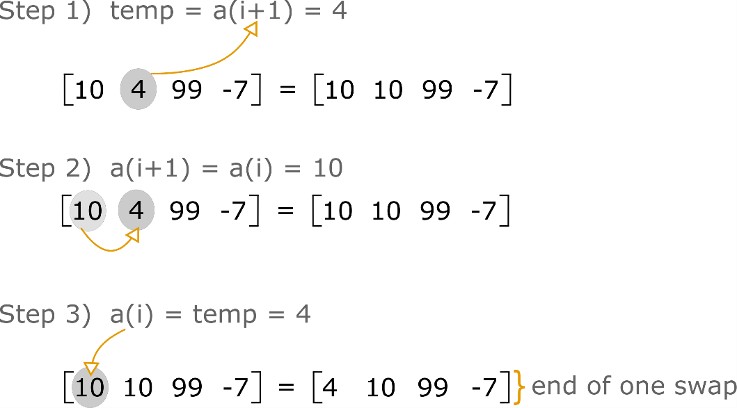
Figure 1: Visualization of how two elements are swapped in the bubble sort method.

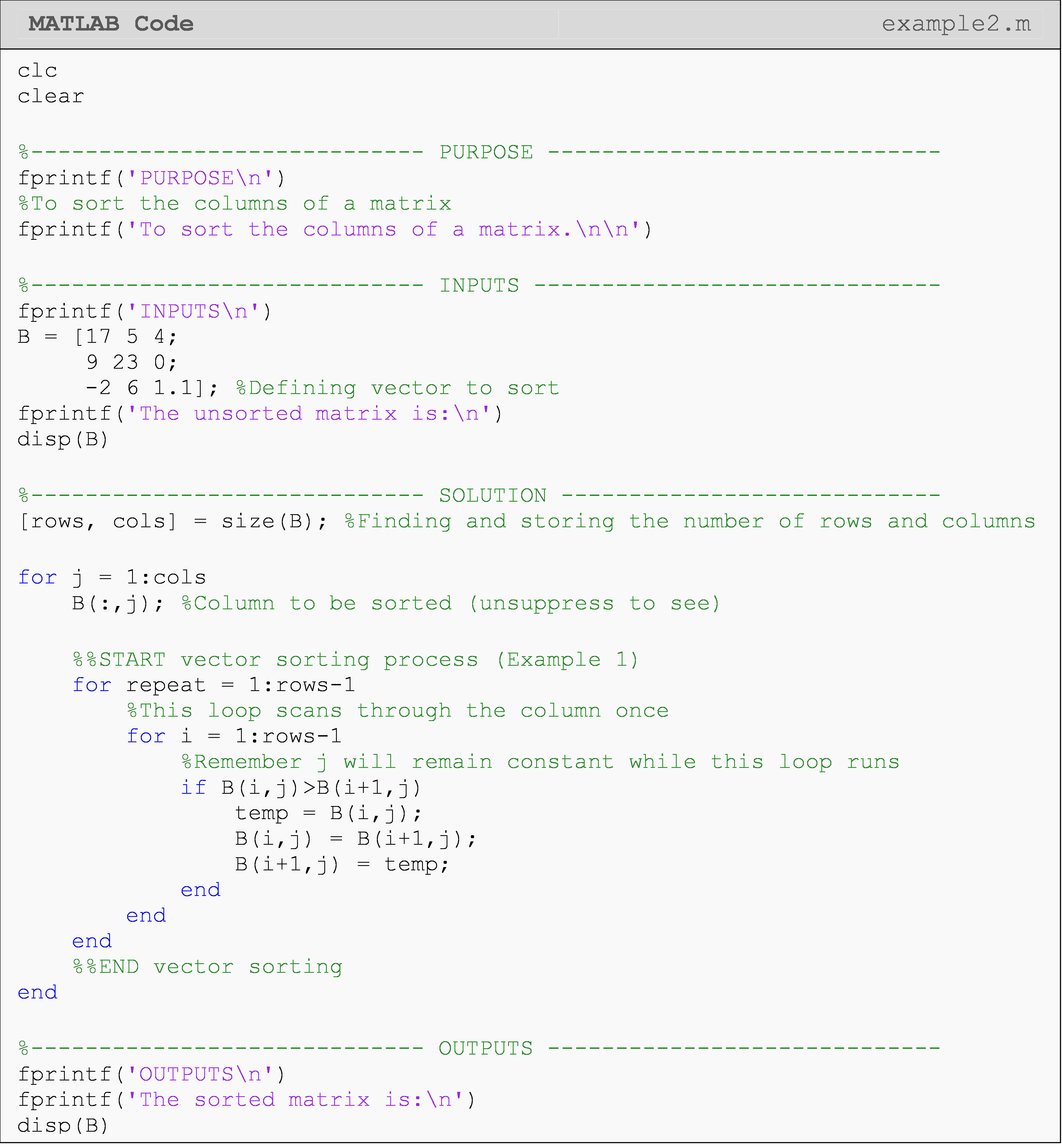
In Example 2, we will apply the ideas covered in Example 1 to a matrix. As noted in the example, this is as simple as adding another for loop to repeat the process for each “vector” (row or column depending on your choice) in the matrix.

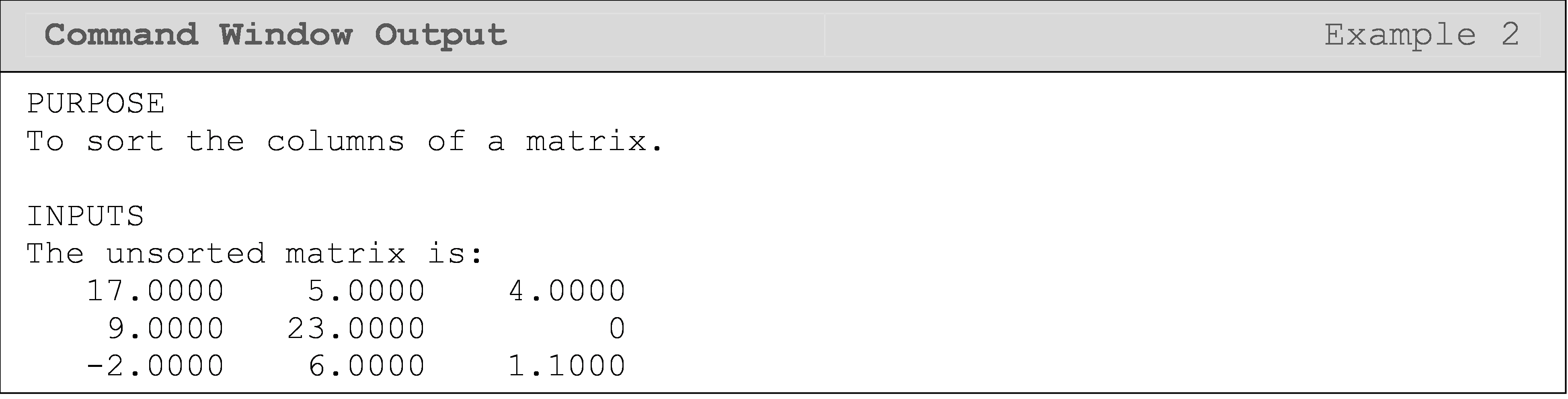
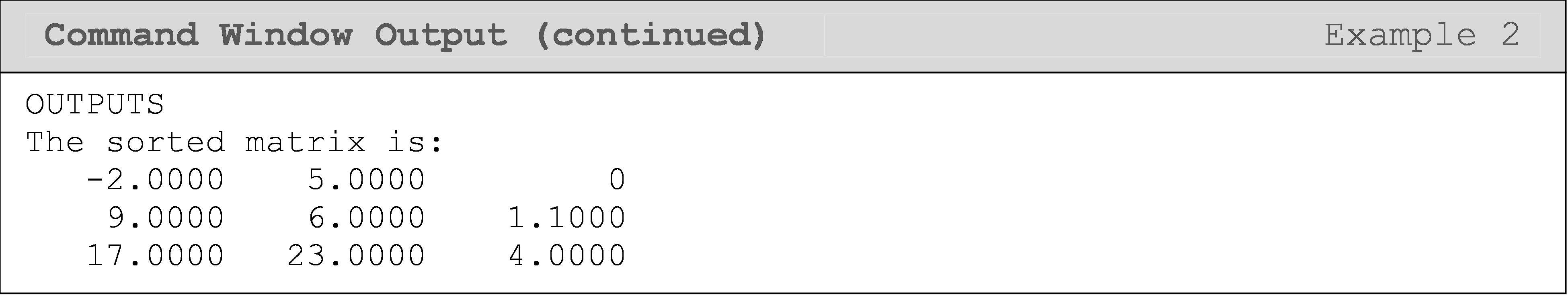
Example 2

Sort the columns of any given matrix. Test the solution using matrix [B].

\[[B]=\displaystyle\begin{bmatrix}17 & 5 & 4 \\ 9 & 23 & 0 \\ -2 & 6 & 1.1 \\ \end{bmatrix}\]

Treat each column as a vector. All we need to do is repeat the vector sorting process for each column in the matrix. Therefore, we only need to nest Example 1 inside another loop.

Solution

How can I find the sum of a vector?

It is relatively simple to find the sum of a vector manually, and there is even a built-in MATLAB function for it called sum(). In fact, we have already covered summing in a loop when we covered while loops (Lesson 8.1). However, it is important to pay close attention to the next example as it takes advantage of a key property of loops to create a summing mechanism, which is itself extremely common.

Example 3

Find the sum of any given vector. Do not use the built-in MATLAB functions such as sum().

Test the program with the vector: \([a] = [1\ \ 565\ \ 4\ \ 5\ \ 8\ \ 9\ \ 22]\).

Solution

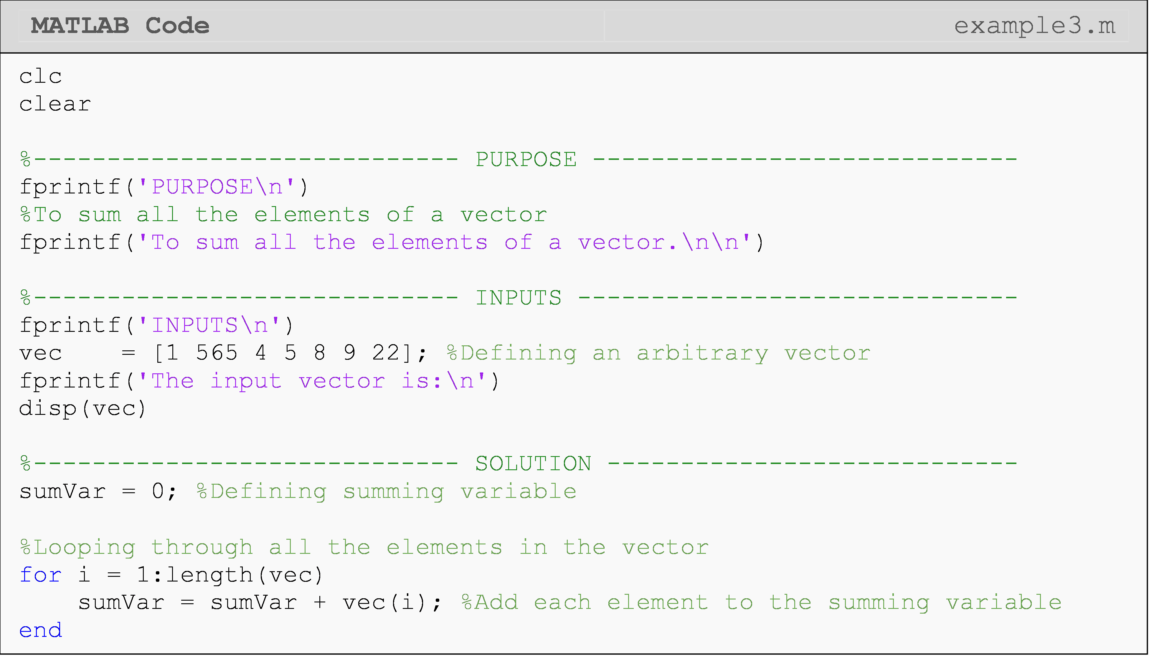
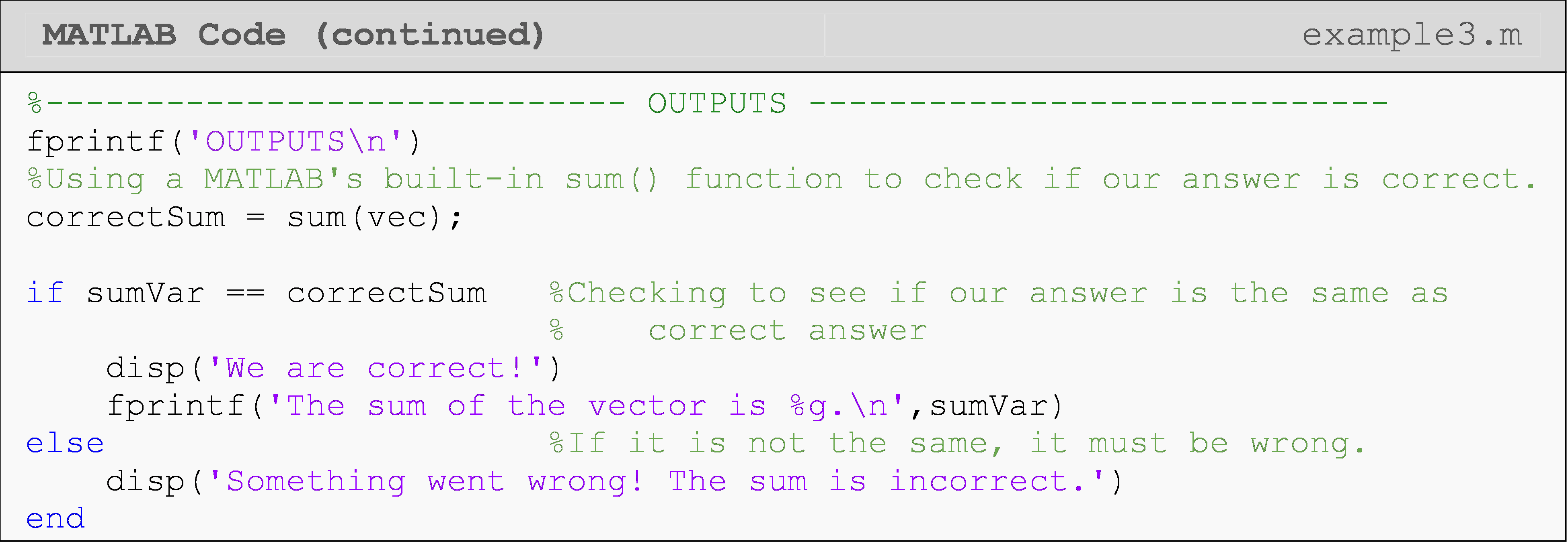
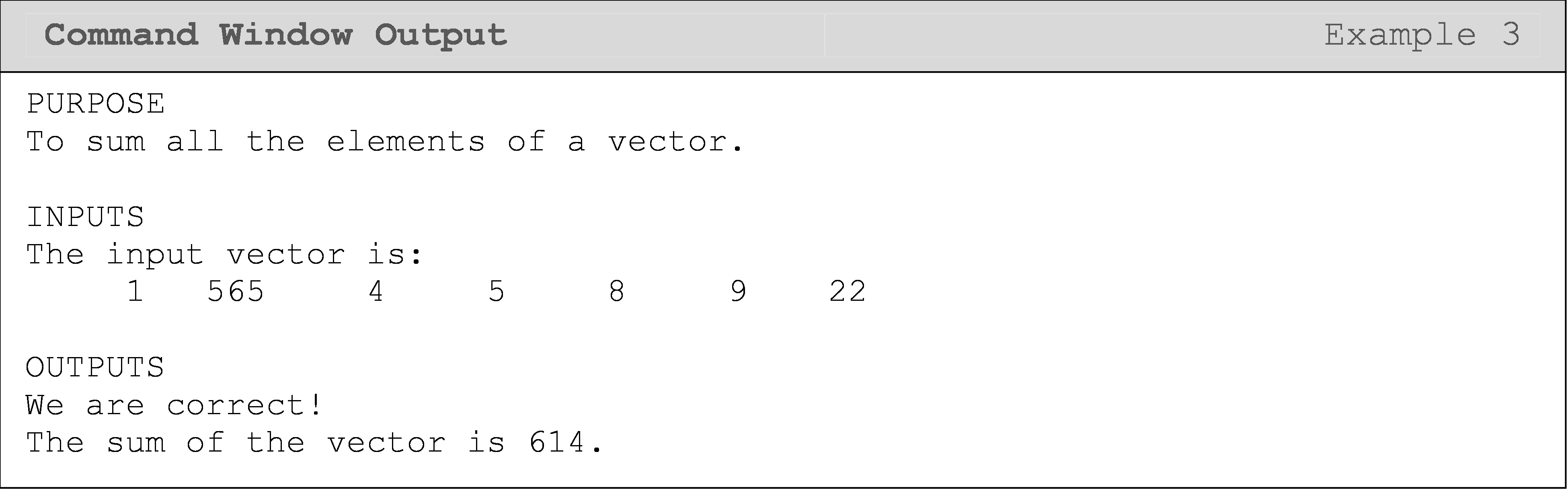
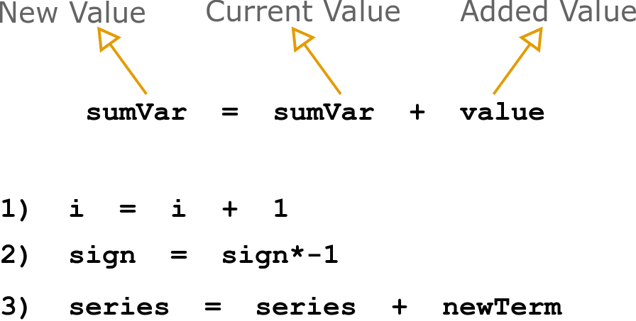Figure 2: General form of changing the current value of a value and update the variable to the new value. Below that, you can see three applications of the concept.

Some use cases for calling a variable and assigning it a new value on the same line (see also Figure 2) are:

i = i + 1
sign = sign*(-1)
series = series + newTerm

One can see that the same fundamental concept of calling and assigning variables is used in each case. When a variable appears on the right side of the equals sign, the variable is being called (we are asking for its current value). When a variable appears on the left side of the equals sign, we are assigning the variable a new value. One needs to fully grasp this concept.

You can get more practice with summing things in a loop by using different types of series. Also, remember summing can be implemented in a matrix by recognizing that matrices are just collections of vectors (columns/rows depending on how you would like to sort).

How can I plot different variations of a function using loops?

In some cases, we need to plot many different sets of data points, and to avoid long chains of plot() calls, we can use loops to run one plot() call multiple times. (If you need a quick review on plotting, jump to Lesson 3.1.) A few examples of this are changing part of an equation, hence, changing the vector of data and the equation to the plot. Example 6 shows the first of these cases where we multiply a function by a different constant in each iteration and show them all on the same plot (Figure 3).

Important Note: In general, you should avoid placing lines of code inside loops that never change between the beginning and end of the loop as this would make your code less efficient.

Example 4

Using only one plot() call and a for loop, plot the mathematical function, \(y(x)=ke^x\) from \(x = 0 \text{ to } 6 \text{ for } k=1,2,...,5.\)

Solution

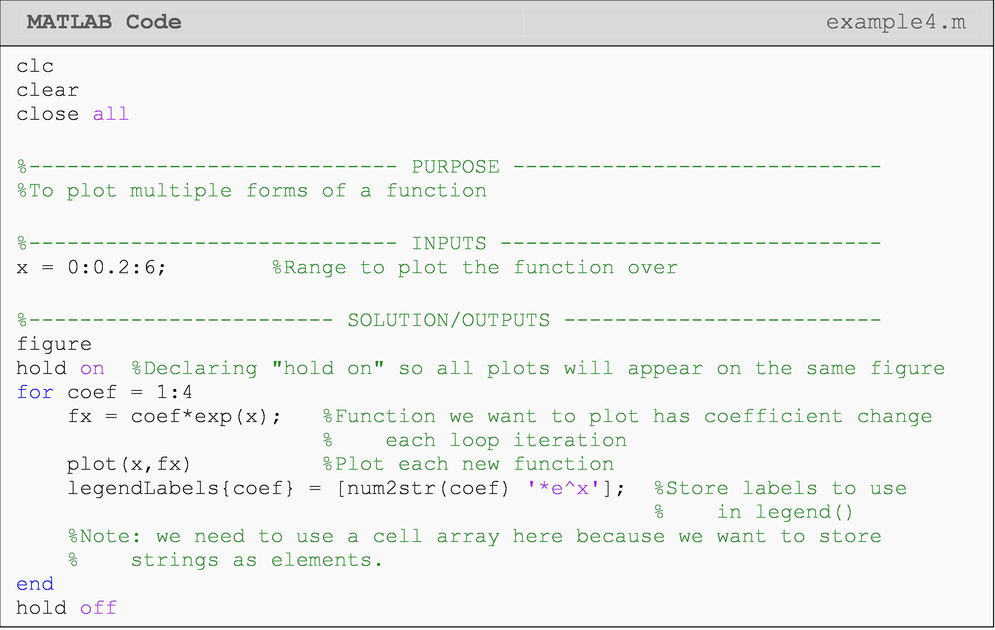
As shown in Figure 3, all five functions are plotted on one plot. One can see that as the value of k increases, the slope of the function increases. To get appropriate legend labels in an automated way, we make use of cell arrays, which are, in structure, like the vectors and matrices we are familiar with except cell arrays can hold non-numeric values like strings of text.

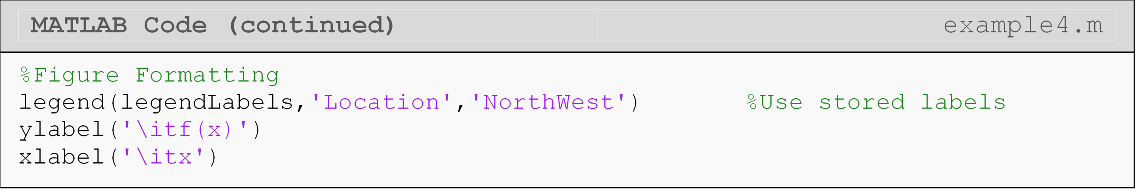
To create our legend on the plot, we simply assign legend() our cell array of strings. If you do not fully grasp the concept of a cell array, that is ok because it is not the focus of this lesson.

!](./Chapter0806Lesson100AppliedLoopsMedia/media/image5.png){width=“3.7604166666666665in” height=“2.967199256342957in”}
Figure 3: Figure output for the code given in Example 4.

Although this lesson is certainly not an exhaustive list of common techniques you might use in loops, it should give you an idea of what to be on the lookout for. This module should also serve as a lesson in how important experiential programming skills are.

In the first half of the module, we introduced new syntax related to the fundamental programming concept of loops (iterating code). In the second half of this module, we have covered many different programming solutions using loops that covered important skills and knowledge but without introducing much new syntax. This should encourage and motivate you to commit these and any other programming techniques to memory.

Multiple Choice Quiz

(1). The Command Window output of the following program is

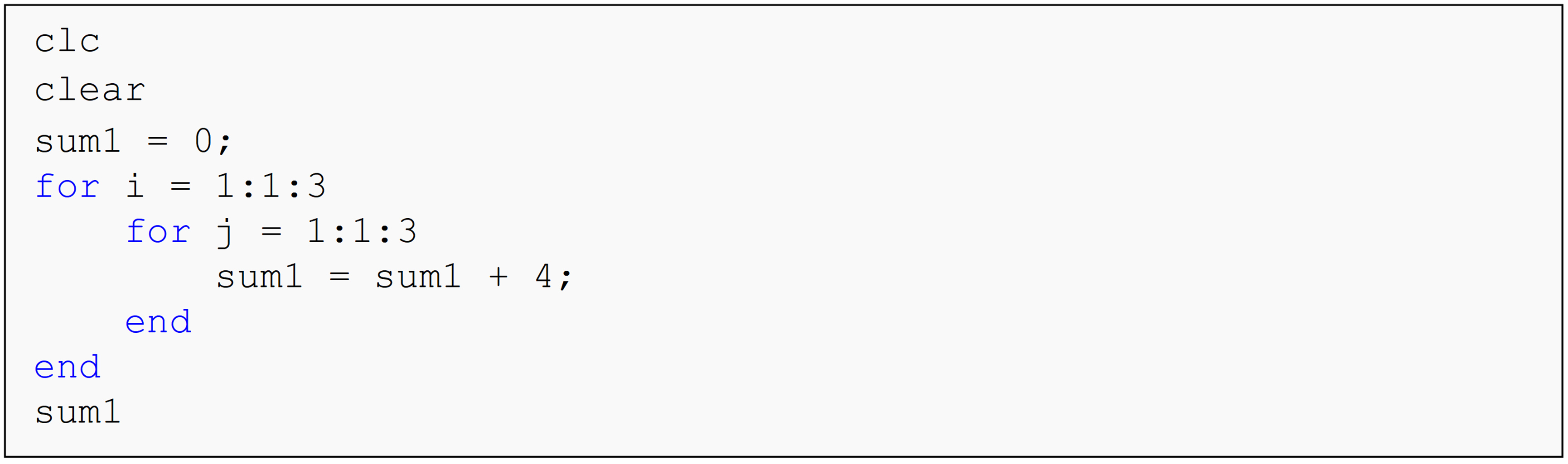
(a) sum1 = 0

(b) sum1 = 4

(d) sum1 = 36

(2). The Command Window output of the following program is

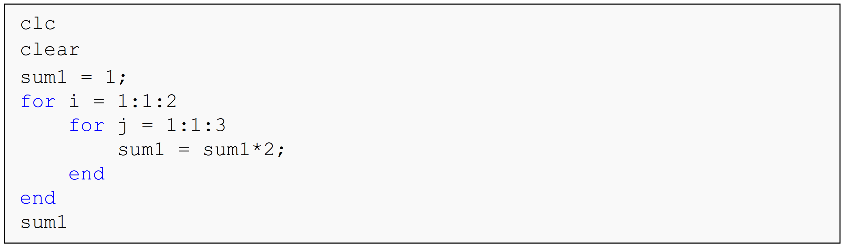
(a) sum1 = 18

(b) sum1 = 64

(d) sum1 = 128

(3). The Command Window output of the following program is

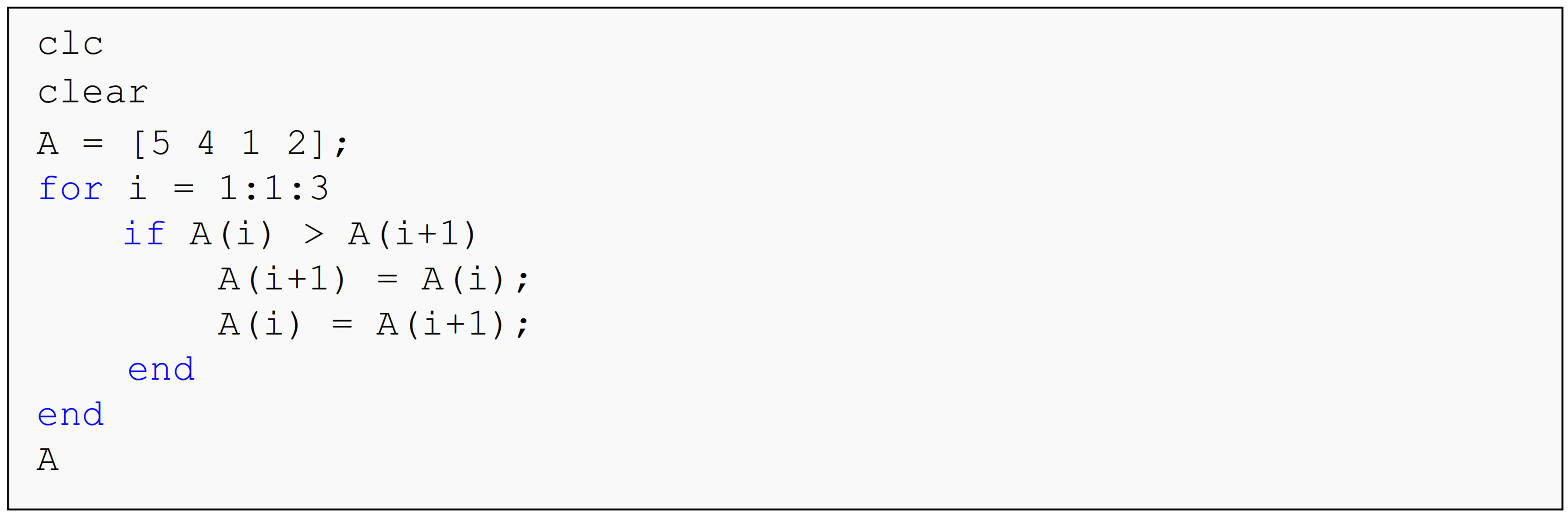
(a) A = [4 1 2 5]

(b) A = [5 4 1 2]

(d) A = [1 2 4 5]

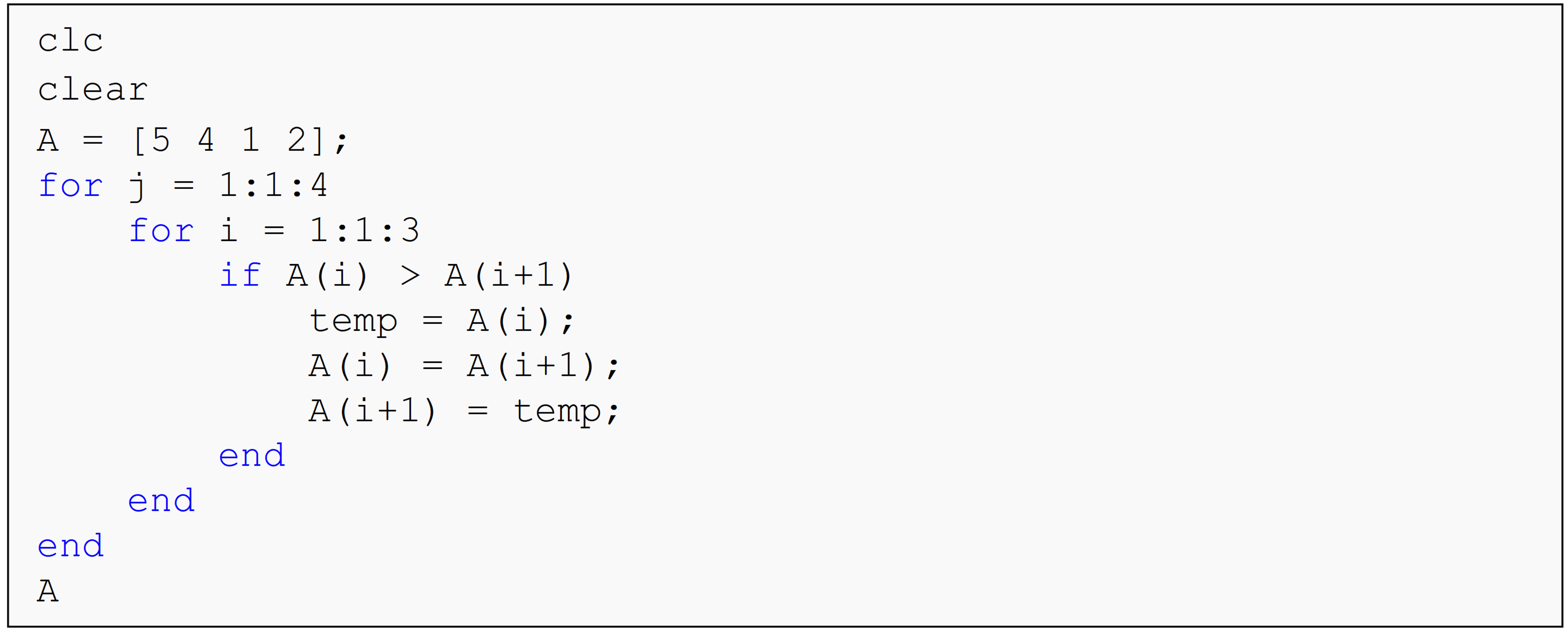
(4). The Command Window output of the following program is

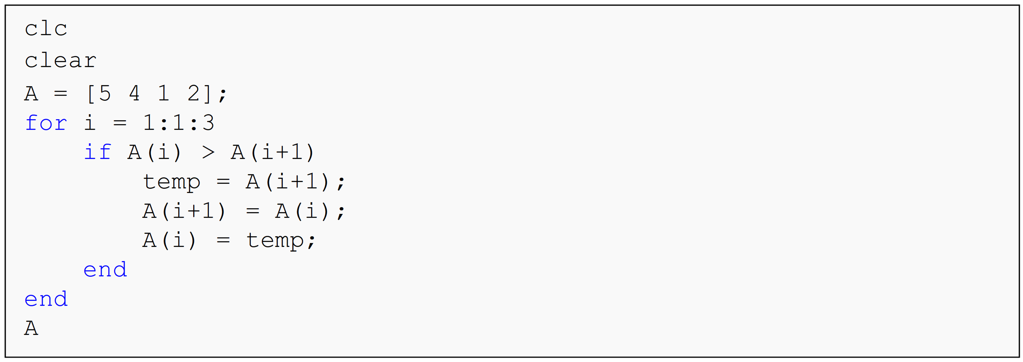
(a) A = [4 1 2 5]

(b) A = [5 4 1 2]

(d) A = [1 2 4 5]

(5). The Command Window output of the following program is

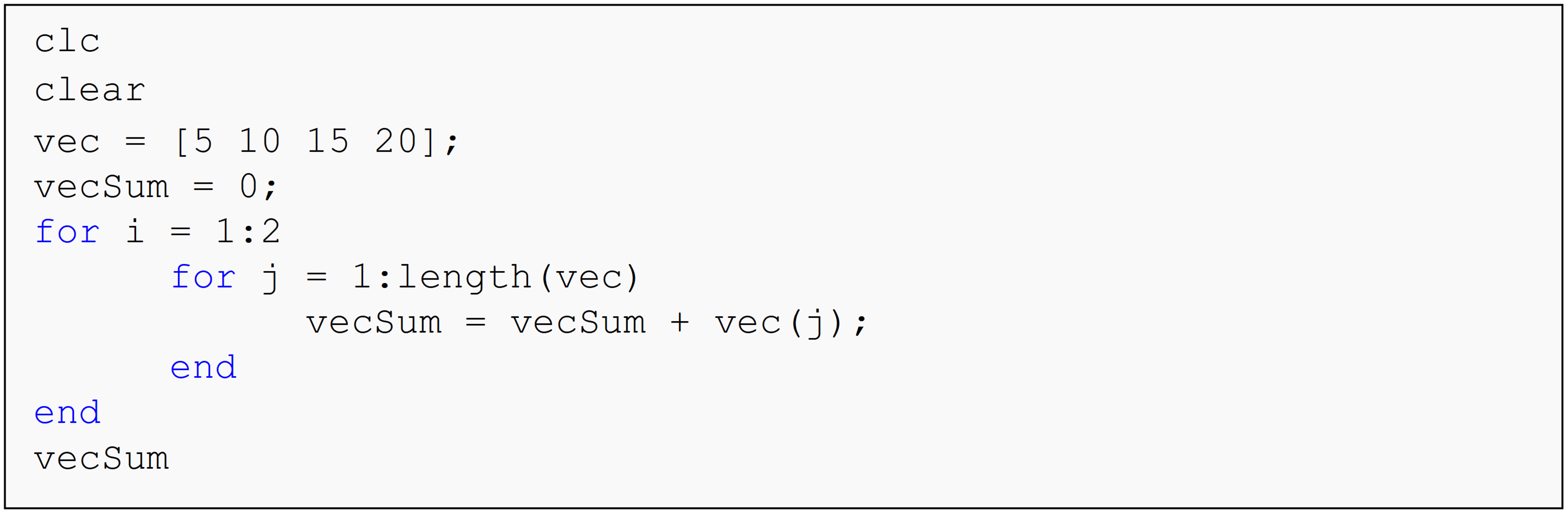
(a) vecSum = 50

(b) vecSum = 150

(d) Undefined function or variable 'vecSum'.

(6). The Command Window output of the following program is

(a) A = [4 1 2 5]

(b) A = [5 4 1 2]

(d) A = [1 2 4 5]

Problem Set

(1). Using your knowledge of loops and/or conditional statements, write a MATLAB program that determines the value of the following infinite series

\({f}({x}) = {x} + \displaystyle\frac{{1}}{{2}}{x}^{{2}} + \frac{{1}}{{3}}{x} + \frac{{1}}{{4}}{x}^{{2}} + \ldots\).

There are two program inputs

the value of x, and
the number of terms to use.

There is one program output

the numeric value of the series.

Your program must work for any set of inputs. Assume that the value for the number of terms to use will always be entered as a positive whole number.

Test your program for the following set of inputs:
number of terms = 26
value of x = 0.67

(2). Write a program to numerically sort any input vector, vec, from smallest to largest. You may use the bubble sort program shown in Example 1 of this lesson as a guide. Test and run your program for the following vector vec = [8, 2, 16, 12, 2, 5].

(3). Write a program to numerically sort any input vector, vec, from largest to smallest. You may modify the bubble sort program shown in Example 1 of this lesson. Test and run your program for the following vector vec = [8, 2, 16, 12, 2, 5].

(4). A typical alarm clock has the following features: (1) alarm set time, (2) current time, and (3) desired “snooze” time. Use your knowledge of loops (for-end and/or while-end) and conditional statements to write a MATLAB program that outputs the wake up time of an individual using an alarm clock. The program inputs are:

Alarm set time (disregard AM and PM setting), alarmSet as a vector with 1 row and 2 columns, with the first element being the hour and the second element being the minutes.
Initial “snooze” time, snooze. (This time value is always \(\geq\) 4 minutes)
Number of times the “snooze” button is used, n. (\(0 \leq n \leq 50\))

Each time the snooze button is used after the first use, the snooze time decreases by 1 minute. However, the minimum snooze time is 4 minutes.

The program output is (after the snooze button is hit n times):

Final wake up time, wakeup as a vector with 1 row and 2 columns, with the first element being the hour and the second element being the minutes.

Test the program using this example: If the alarm set time is at 7:30 and is entered as alarmSet = [7 30], the initial snooze time is set at 8 minutes, and the snooze button was hit 6 times, the wake up time is 8:04 (overall snooze time is: 8+7+6+5+4+4=34), hence wakeup = [8 4].

(5). Using your knowledge of loops and/or conditional statements, write a MATLAB program that conducts the following summation,

\[\sigma = \sum_{{j} = {1}}^{{n}}\left( {ax}{(}{j}{)} + {e}^{{y}{(}{j}{)}} \right)\]

where,

\[a = \text{real constant}\] \[y = 0.367aj\] \[x = \displaystyle\left\{\begin{split} &4.5y + 0.5jy < 2 \\ &jy \geq 2 \end{split}\right.\]

The program has two inputs, the number of terms to use, n and the value of the constant, a. The program has one output, the numeric value of the summation. Do not use the sum or similar MATLAB function to complete this problem.

Test and run your program for the following set of inputs: a = 0.75 and n = 30.

(6). Without using the max(), min(), or sort() functions, write your own MATLAB program that finds the minimum and maximum element of any input vector. Output the original vector, and the minimum and maximum elements. Test your program for the following input vector vec = [12, 9, -10, 8, 8.9, -7.8, 15].

(7). The secant method is used to approximate the value of the root(s) of an equation f(x)=0. The secant method requires the user to make two initial guesses x₀ and x₁ of the root of the equation, but which do not necessarily need to bracket the root. The secant method iterative formula is given by

\[\displaystyle {x}_{{k} + 1} = {x}_{{k}} - \frac{{x}_{{k}} - {x}_{{k} - 1}}{{f}\left( {x}_{{k}} \right) - {f}\left( {x}_{{k} - 1} \right)}{f}\left( {x}_{{k}} \right),\ \ {k} = {0,1,2,3,}{…}\]

where,
\({x}_{{k}{+1}}\) is the current approximation,
\({x}_{k}\) is one of the previous approximations,
\({x}_{k - 1}\) is the other previous approximation.

This process is repeated until the root is found.

Write a program that uses the secant method to find the approximate root(s) of an equation. The program inputs are, the function f, the first two guesses, x(1) and x(2), and the number of iterations to conduct, n. The output is the approximate value of the root of the equation, rootVal.

Although not required, use vectors to store the approximations of the root. Your developed vector will contain n+2 elements.

Hint: Be sure not to use same numbers for the initial two guesses, and only use a reasonable number of loop repetitions.

(8). Without using the max(), min(), or similar MATLAB functions, write a program that outputs the maximum and minimum element values of any rectangular matrix.

The program input is:

a rectangular matrix, mat.

The program outputs are:

the maximum value, big, and
the minimum value, small.

Test and run your program for the following matrix, mat.

\[\begin{bmatrix} - 1 & 0 & 2 \\ 7 & - 4 & 12 \\ 4 & 8.2 & 11 \\ - 11 & 0 & - 12 \\ \end{bmatrix}\]

(9). Write a program in MATLAB that for a square matrix subtracts the sum of the absolute value of the elements above the diagonal from the product of the absolute value of the diagonal elements. Do not use the sum() or any other similar MATLAB functions to solve this problem. Use your knowledge of loops and/or conditional statements to write the program.

The program input is:

a square matrix, A.

The program output is:

the value of the difference, processedMat.

Test and run your program for the following \({4} \times {4}\) matrix, A.

\[\begin{bmatrix} 3 & 7 & 10 & - 15 \\ 3 & - 1 & 5 & 0 \\ 66 & 11 & 5 & 1 \\ 0 & - 5 & 2 & 2 \\ \end{bmatrix}\]

Hint:
The product of the absolute value of the diagonal terms is
\(= \left| {3} \right| \times \left| - {1} \right| \times \left| {5} \right| \times \left| {2} \right| = {30}\).

The sum of the absolute value of the terms above the diagonal is
\(= \left| {7} \right| + \left| {10} \right| + \left| - {15} \right| + \left| {5} \right| + \left| {0} \right| + \left| {1} \right| = {38}\)

The value processedMat for the above matrix is \(= 30 - 38 = - 8\).