Module 4: MATH AND DATA ANALYSIS
Learning Objectives
After reading this lesson, you should be able to:
solve linear equations in MATLAB,
solve nonlinear equations in MATLAB,
manipulate polynomials and polynomial coefficients,
plot data with the syms data type.
How do I solve for roots of a linear equation?
In this section, we will go over using MATLAB to solve for the roots of
an equation using
solve(). For
example, \(x-2=0\) has a root at \(x=2\).
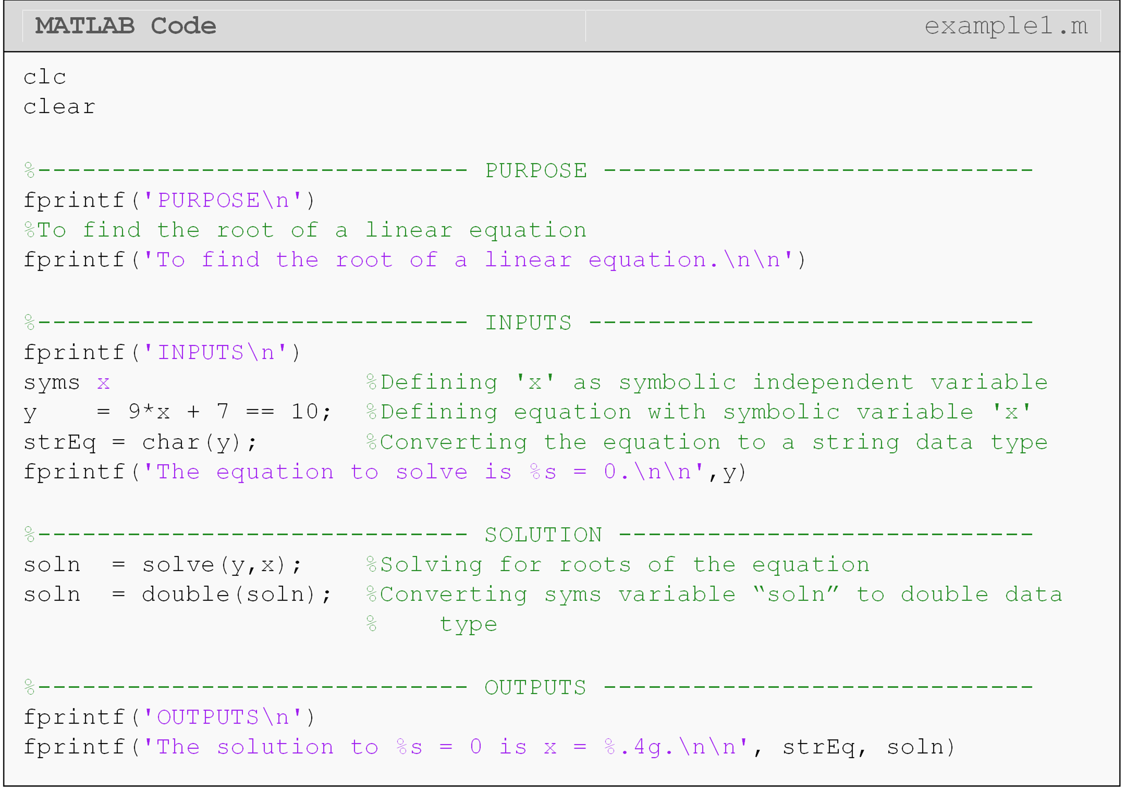
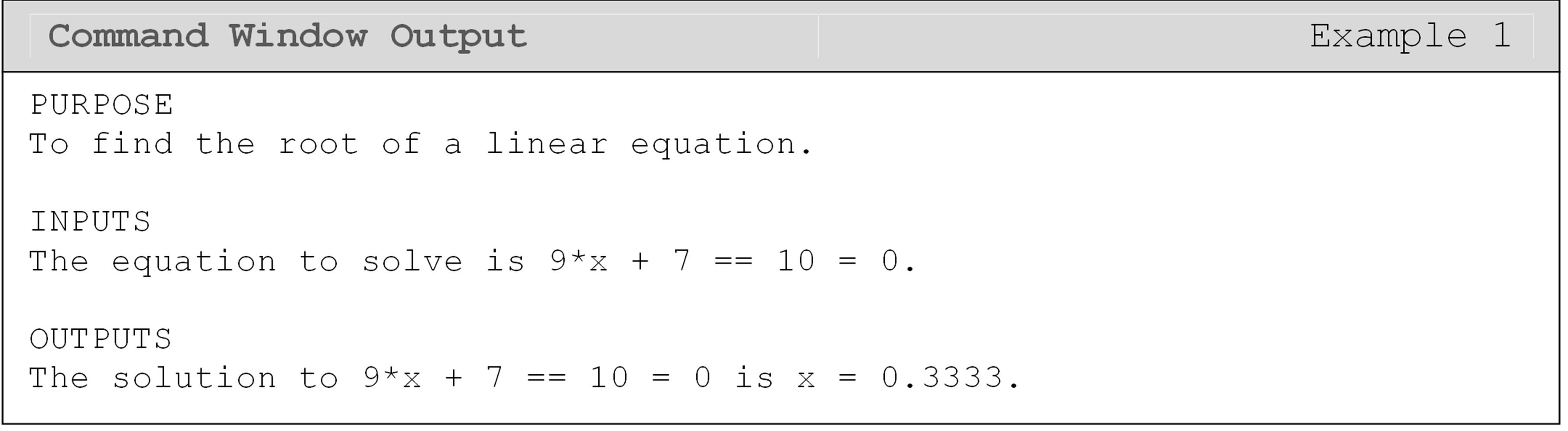
Example 1 shows the procedure for solving for the root of a linear
equation in MATLAB. Note that when the equation is defined in Example 1,
we write y = 9*x +7 == 10. This means that the equation
9*x + 7 == 10 is stored in the variable y, which we call subsequently
in the program like we would any other variable. The right-hand side of
the equation that you enter does not have to be equal to zero. For
example, you could also write 9*x == 3 and still get the same answer
from MATLAB.
You might be asking at this point, “Why do we need double equals when
entering the equation?” The simple answer to this is that MATLAB needs
to recognize that you are entering an equation rather than storing
something in a variable. Remember that y = 9*x + 7 == 10 has two
parts. Entering the equation 9*x + 7 == 10 is stored in the variable
y. MATLAB needs a way to differentiate between these two operations. All
you need to remember is to put the double equals (==) when entering an
equation. MATLAB will return an error if you fail to do so.
What is a nonlinear equation?
A nonlinear equation is an equation that has nonlinear terms of the unknowns. One of the simplest examples of a nonlinear equation is the quadratic equation that has the form
\(ax^{2} + bx + c = 0\) (1)
where,
\(a \neq 0\).
The values of a, b, and c are constant coefficients and x is the independent variable. If one were to solve a nonlinear equation using traditional methods they would need to be provided at least two items: the nonlinear equation and the unknown variable to solve for.
Take the case of the equation given in the above Equation (1). The nonlinear equation is a quadratic equation and the variable to solve for is x. This example can be solved using the widely known solution of a quadratic equation as
\(x = \displaystyle\frac{- b \pm \sqrt{b^{2} - 4ac}}{2a}\) (2)
However, other more complex nonlinear equations can take longer to solve exactly, while most nonlinear equations are impossible to solve analytically. Another example of a nonlinear equation is \(\text{sin}(2x) = \displaystyle\frac{3x}{7}\). In these cases, MATLAB can be used to solve the nonlinear equations or even to verify the results obtained from an analytical method.
How can I use MATLAB to solve nonlinear equations?
As we know, MATLAB is a tool. Just like a mechanic might use a wrench to solve a problem, an engineer, scientist or mathematician might use MATLAB to solve a problem. In the case of solving a nonlinear equation, MATLAB can be used to solve nearly any equation (limited more so by the operating computer than the program itself).
We used solve() to find the roots of a linear equation as a
demonstration of symbolic variables. However, solve() is also used to
find the roots of nonlinear equations. In this case, we may get multiple
roots. Unique, none and infinite number of solutions are other
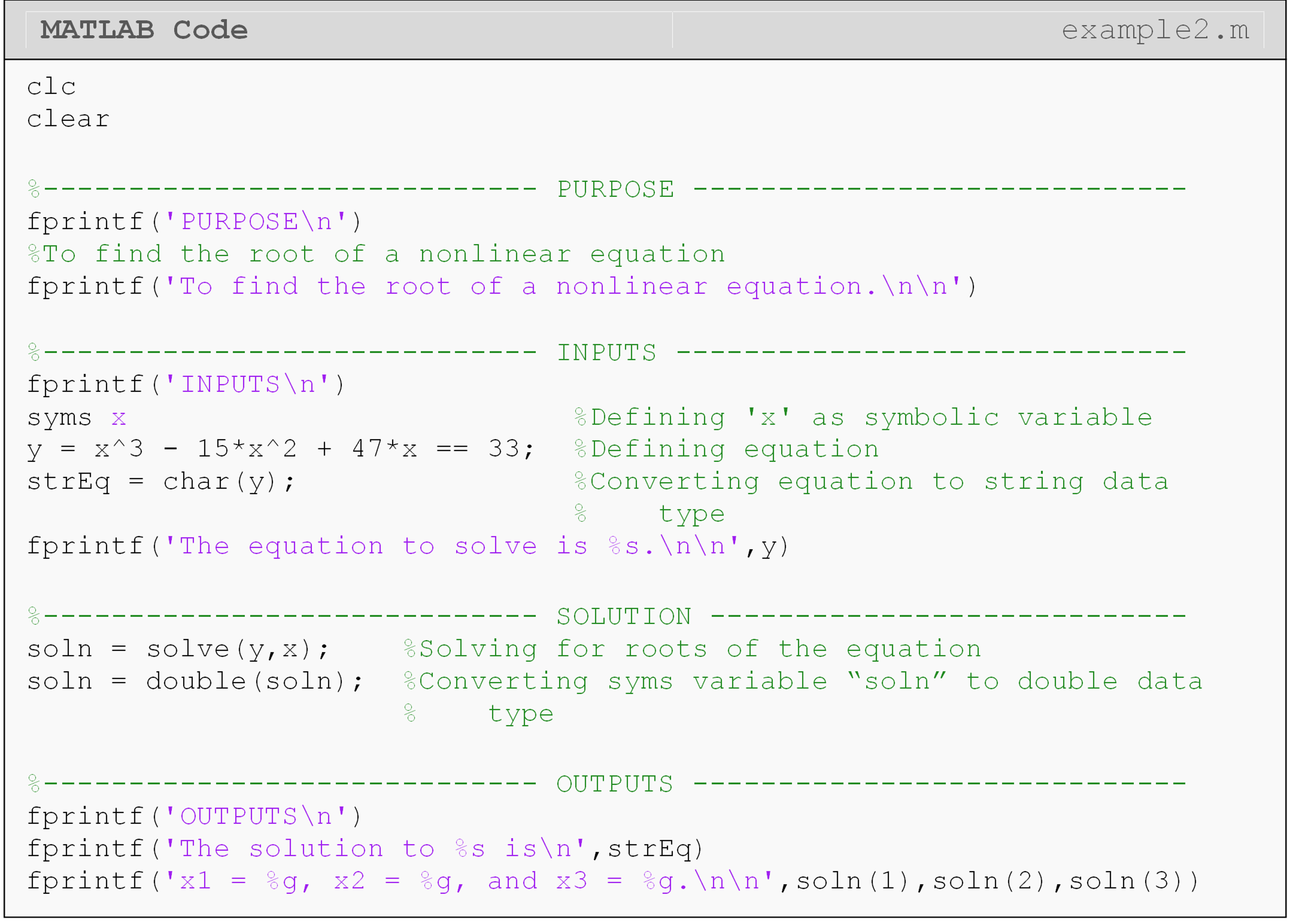
possibilities for nonlinear equations. Multiple roots will be stored in
vector form, which you can see in Example 2. The variable soln is a
vector that holds the three roots we found from the third-order
polynomial equation.
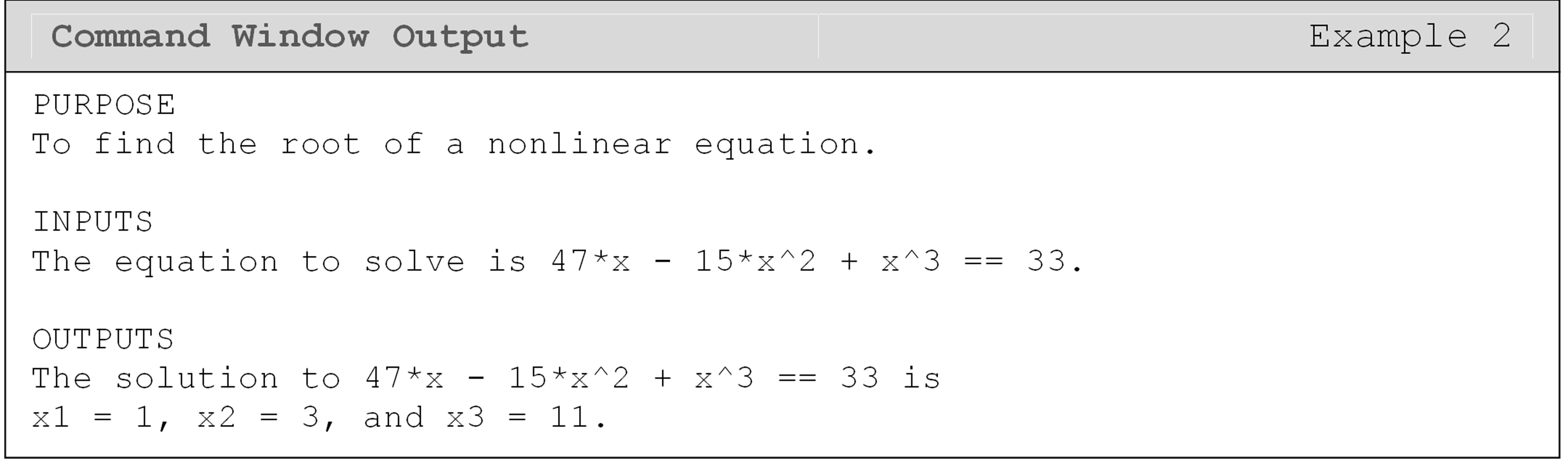
You can see in Example 2 that the solution to the nonlinear equation has three possible values. We know this is correct because the equation is a cubic equation. The outputs to the solve command are stored in a vector and can each be pulled out of the vector by using matrix references, which we covered in Lesson 2.6.
Example 2
Solve the nonlinear equation \(x^3-15x^2+47x=33\) for x using MATLAB (that is, find its roots).
Solution
MATLAB also provides a method to solve an equation numerically using
vpasolve()
(note that solve() uses analytical methods). Although polynomial
equations have a finite number of solutions (which is equal to the order
of the polynomial), other nonlinear equations can possibly have an
infinite number of solutions (e.g., \(\text{tan}\left(x \right) = x\)).
Therefore, MATLAB does not report all solutions in the same way. Check
the
vpasolve()
documentation for specifics.
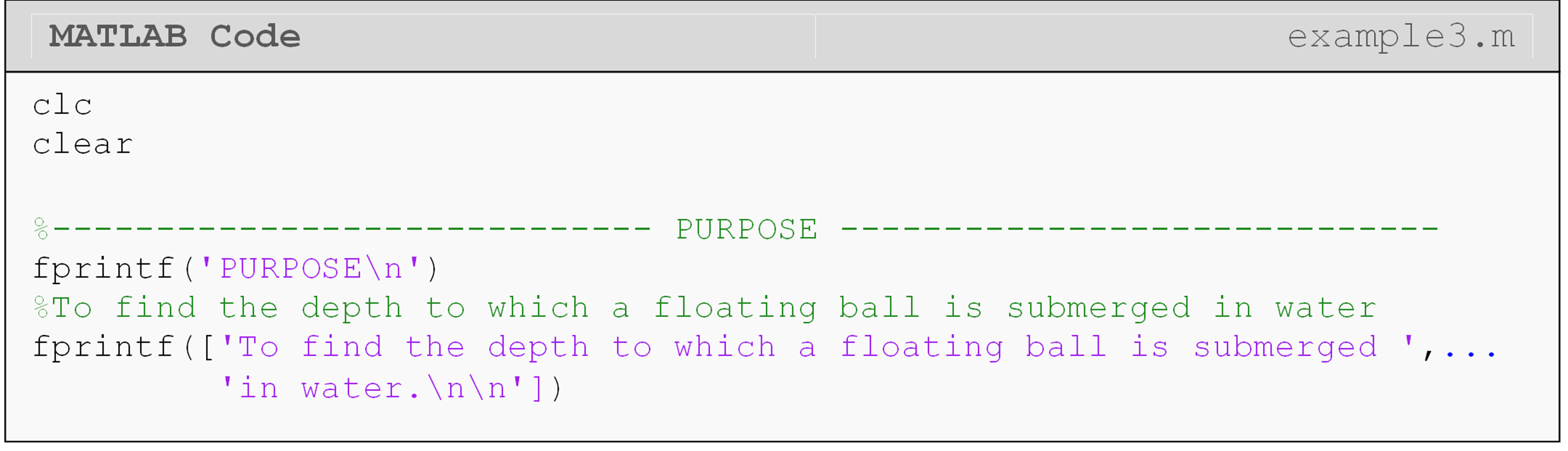
In Example 3, we show an application that shows a real-world problem.
The only difference here is the prerequisite mathematical knowledge to
set up the problem (find the appropriate equation). The programming
portion is more or less the same, which is the beauty of MATLAB and many
other similar programming languages. Once written, a program like the
one in Example 2 can be quickly edited for a completely different
equation like the one in Example 3. We chose to use the aforementioned
vpasolve()
in Example 3.
Example 3
Find the depth x to which a ball is floating in water (see Figure 1) based on the following cubic equation
\[4R^{3}S - 3x^{2}R = - x^{3}\]
where,
R = radius of the ball,
S = specific gravity of the ball.
Use values of R and S to be 0.055 and 0.6, respectively.
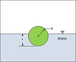
Figure 1: Diagram of a partially submerged sphere in water for use with Example 3.
Solution
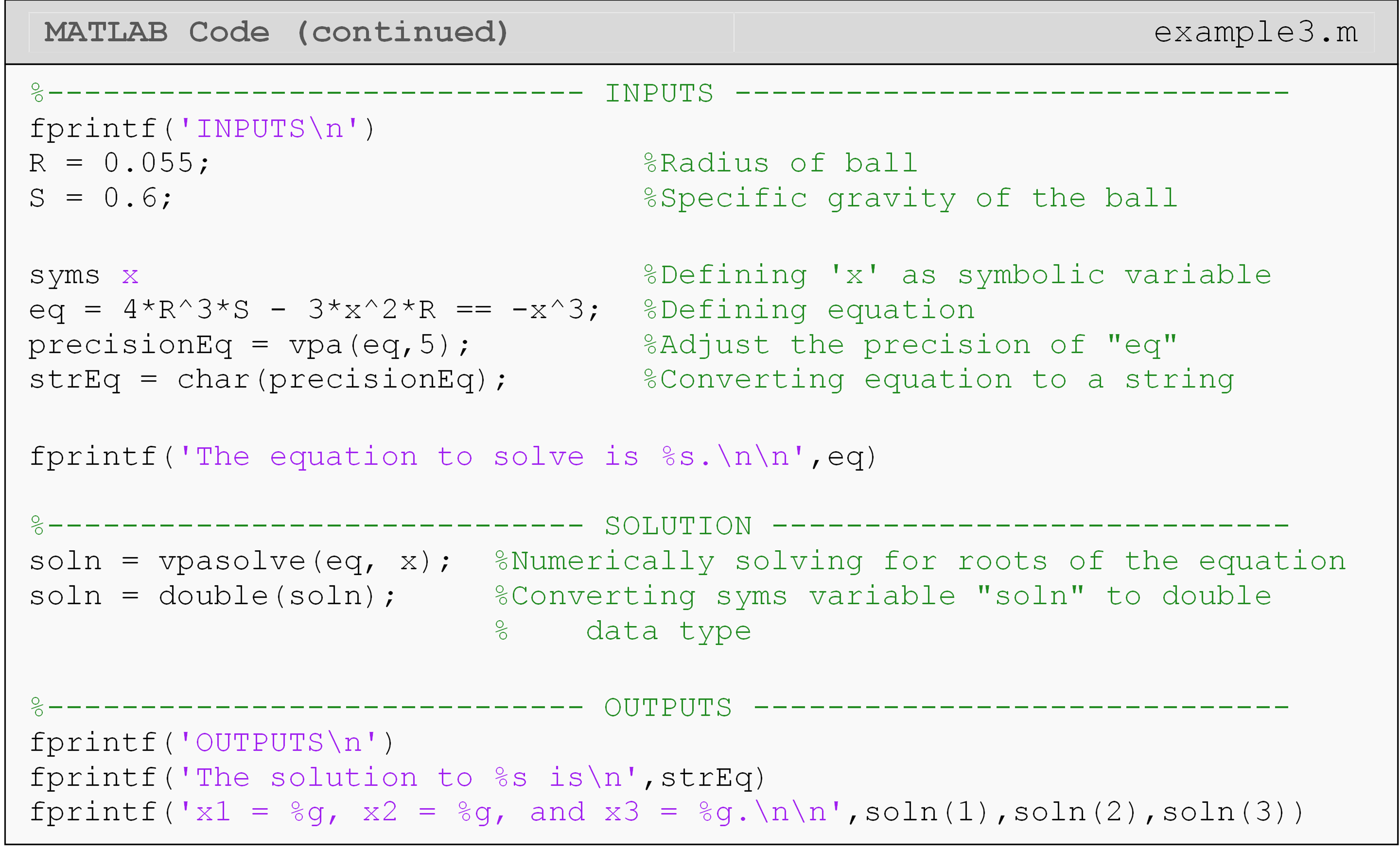
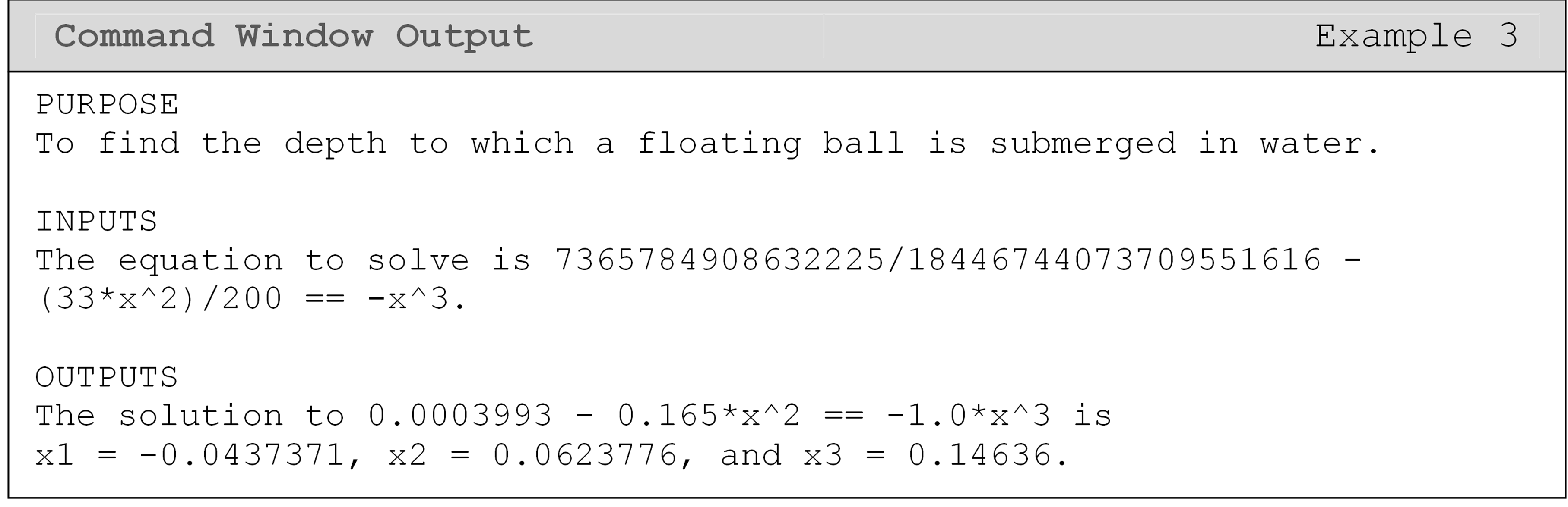
Note the three possible solutions to the third order polynomial equation for Example 2. Since the limits of x are given by \(0 \leq x \leq 2R\) and R = 0.055, the limits of x are \(0 \leq x \leq 0.11\). Hence, the only physically acceptable solution is \(x = 0.0624\).
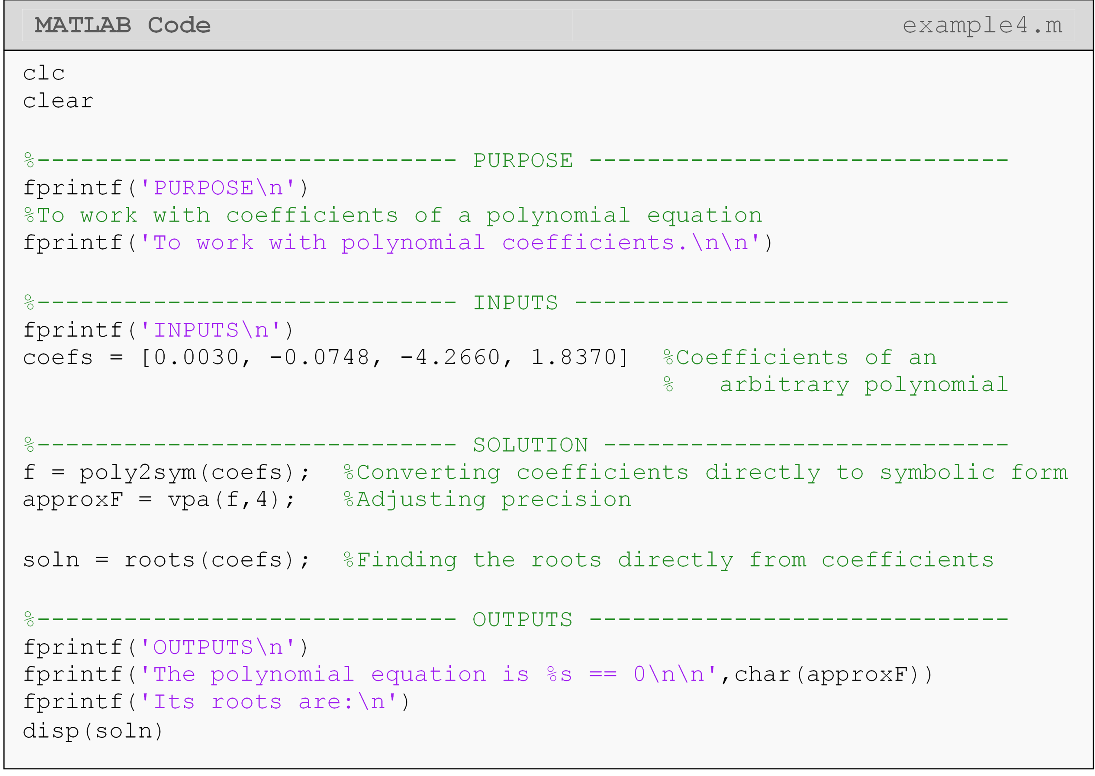
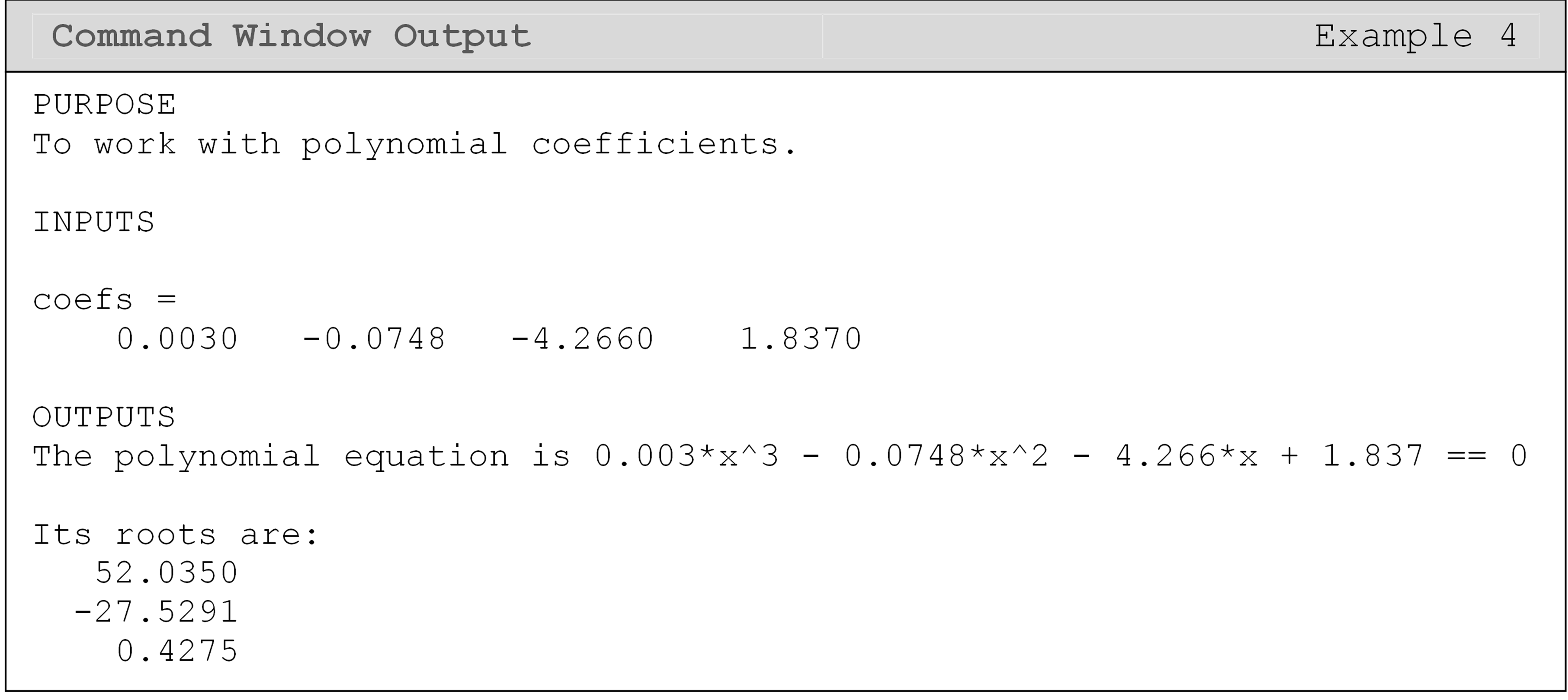
Is there a faster way to work with polynomial equations in MATLAB?
We can create a symbolic polynomial from a vector of coefficients using
the function
poly2sym().
(You can do the reverse operation with
sym2poly().)
This can be especially helpful when using functions that return a vector
of coefficients directly such as
polyfit(),
which we will cover later in Lessons 4.7 and 4.8. You can see in Example
4 that the coefficient output (coefs) is not very intuitive. However,
we can directly convert the coefficients to polynomial form, which is
more intuitive, and find the roots of the corresponding polynomial with
the
roots()
function.
Can I plot with symbolic variables?
Plotting with
syms has all the
same considerations as any other function you wish to plot with the
additional step of converting to a data type that is accepted by the
function you are using to plot (e.g.,
plot(),
[bar()](https://www.mathworks.com/help/matlab/ref/bar.html?s_tid=srchtitle),
etc.). That is, you will likely need to convert from
sym to a
numeric
data type to plot the data.
To get a vector of data points to plot, we can use the
subs()
function. Although it was used in the previous examples to replace a
variable with just a single number or character, it also accepts vector
inputs as the replacement value(s). When the input is a vector, the
output is a corresponding vector as well.
Example 5
Plot the function \(\displaystyle{y(x)=4x^3-20x^2+9x}\) and its zeros on the same plot. Choose the domain to plot the function based upon the solutions found for the zeros of the function. Include title, axis labels, legend, and plot grid.
Solution
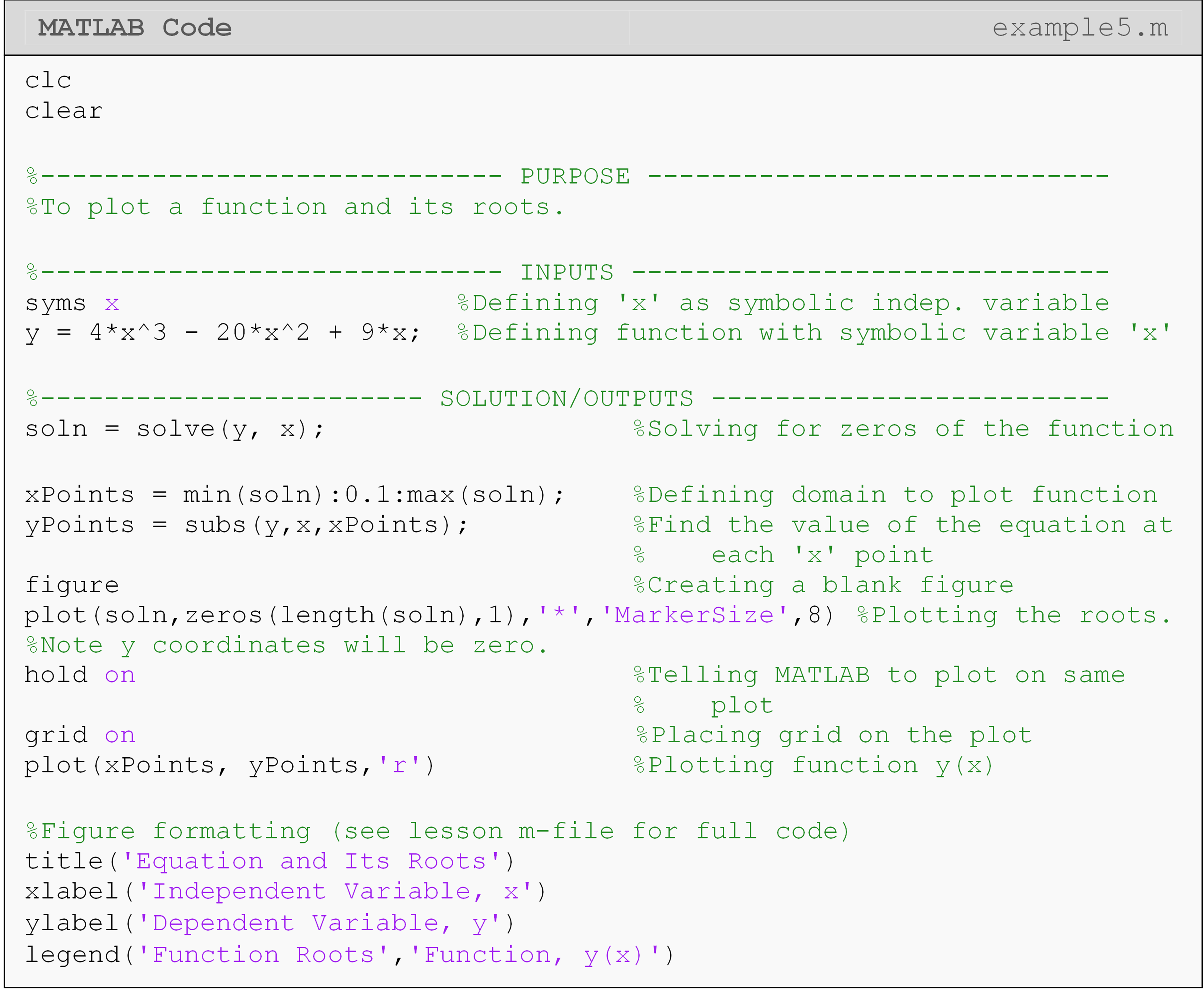
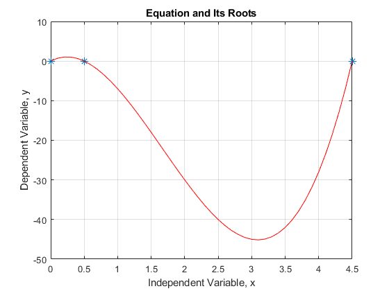
Figure 6: The MATLAB figure output for Example 5.
Lesson Summary of New Syntax and Programming Tools
| Task | Syntax | Example Usage |
|---|---|---|
| Find the roots of an equation | solve() |
solve(eq,x) |
| Numerically find the roots of an equation | vpasolve() |
vpasolve(eq,x) |
| Form a symbolic polynomial function from coefficients | poly2sym() |
poly2sym(coefs,x) |
| Extract the coefficients from a polynomial | sym2poly() |
sym2poly(polynomial) |
| Get the roots of a polynomial using only is coefficients as an input | roots() |
roots(coefs) |
Multiple Choice Quiz
(1). A MATLAB function for solving an equation analytically is
(a) fsolved()
(b) nonlinear()
(c) vpasolve()
(d) solve()
(2). The MATLAB function to find the solution to a polynomial equation given only its coefficients is
(a) solve()
(b) coefs()
(c) roots()
(d) polysolve()
(3). To solve \(x^2+2x=0\), which line of code should be added to the program
(a) solve(x^2+2x==0,x)
(b) solve(x^2-2x,x)
(c) solve(x^2+2*x=0,x)
(d) solve(x^2+2*x==0,x)
(4). The MATLAB substitution function subs() has __________
input variables
(a) 1
(b) 2
(c) 3
(d) 4
(5). The output solutions for a single nonlinear equation given by the
solve() function
(a) gives only one solution to the equation.
(b) gives only the physically acceptable solution(s).
(c) provides the solutions as separate outputs.
(d) stores solutions in a single vector.
Problem Set
(1). Use the solve() function to find the solution of the equation
\(3x^{2} + 2x = 5\). Display the answers in the Command Window.
(2). Given that the value of the two variables a and b can be changed, set up the equation \(ax^{2} + 2x = b\) so that it can be solved for any real values of a and b.
(3). Solve the nonlinear equation \(2x+e^{-x}=5\). Output both the
original equation and at least one of its roots using a single
fprintf() function.
(4). You are working for ‘DOWN THE TOILET COMPANY Inc.’ that makes floats for H3H3 toilets. The floating ball has a specific gravity of 0.6 and has a radius of 5.5 cm. You are asked to find the depth to which the ball is submerged when floating in water (Figure A).
The equation that gives the depth x in meters to which the ball is submerged underwater is given by
\[x^{3} - 0.165x^{2} + 3.993 \times 10^{- 4} = 0\]
Find the depth, \(x\), to which the ball is submerged underwater.

Figure A: Floating ball in water for Exercise 4.
(5). You have a spherical storage tank containing oil (Figure B). The tank has a diameter of 6 ft. You are asked to calculate the height, h, to which a dipstick 8 ft long would be wet with oil when immersed in the tank when it contains 4 \(\text{f}\text{t}^{3}\) of oil. The equation that gives the height, \(h\), of the liquid in the spherical tank for the above-given volume and radius is given by
\[f(h) = h^{3} - 9h^{2} + 3.8197 = 0\]
Find the height, \(h\), to which the dipstick is wet with oil.
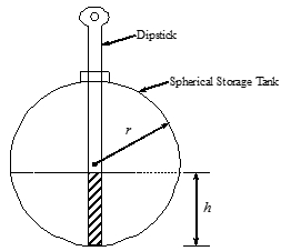
Figure B: Dipstick inside spherical tank which contains some oil. Used in Exercise 5.
(6). You are making a cool bookshelf to carry your interesting books that range from \(8\frac12\)” to 11” in height. The bookshelf material is wood, which has a Young’s Modulus of \(3.667 \text{ Msi}\), length (L) of 29”, a thickness of 3/8”, and width of 12”. You want to find the maximum vertical deflection of the bookshelf. The vertical deflection of the shelf is given by \[v(x) = 0.42493\ \times \text{ 1}\text{0}^{- 4}x^{3} - 0.13533 \times \text{ 1}\text{0}^{- 8}x^{5} - 0.66722\ \times \text{ 1}\text{0}^{- 6}x^{4} - 0.018507x\]
where \(x\) is the position along the length of the beam (Figure C). To find the maximum deflection we need to find where
\[f(x) = \frac{dv}{dx} = 0\]
and conduct the second derivative test. The equation that gives the position,\(x\), where the deflection is extreme (minimum or maximum) is given by \[- 0.67665\ \times \text{ 1}\text{0}^{- 8}x^{4} - 0.26689\ \times \text{ 1}\text{0}^{- 5}x^{3} + 0.12748\ \times \text{ 1}\text{0}^{- 3}x^{2} - 0.018507 = 0\]
(a) Plot the deflection of the beam, \(v(x)\), for values of x from 0 to L.
(b) Find the position \(x\) where the deflection is maximum.
(c) Find the value of the maximum deflection.
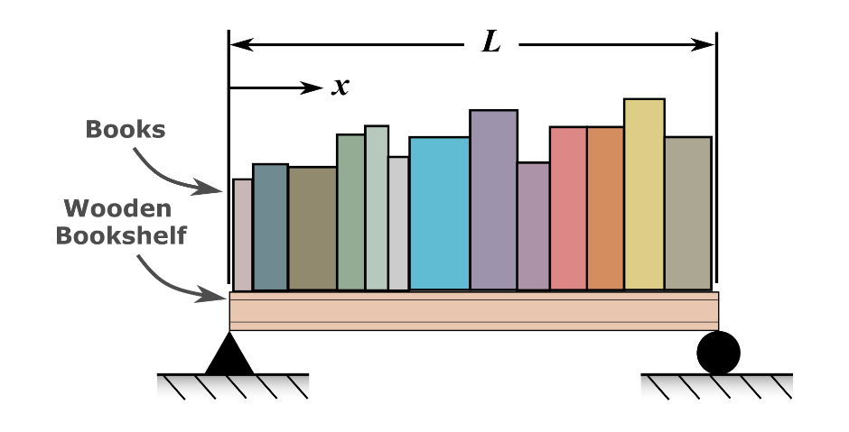 Figure C: Schematic of
bookshelf used in Exercise 6.
Figure C: Schematic of
bookshelf used in Exercise 6.
(d) A trunnion has to be cooled from a temperature of \(80{^\circ}F\)before it is shrink-fitted into a steel hub (See Figure D on the next page). The equation that gives the temperature, \(T_{f}\), to which the trunnion has to be cooled to obtain the desired contraction is given by
\[{f(T_{f}) = - 0.50598\ \times \text{ 1}\text{0}^{- \text{10}}T_{f}^{3} + 0.38292\ \times \text{ 1}\text{0}^{- 7}T_{f}^{2} + }{0.74363\ \times \text{ 1}\text{0}^{- 4}T_{f} + 0.88318\ \times \text{ 1}\text{0}^{- 2} = 0}\]
Find the roots of the equation to find the temperature, \(T_{f}\), to which the trunnion has to be cooled. Choose the physically acceptable root of the equation.
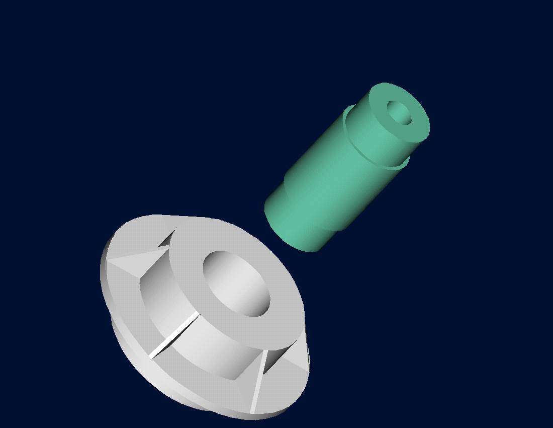
Figure D: Trunnion and hub shown prior to shrink fitting for Exercise 7.