Module 4: MATH AND DATA ANALYSIS

Lesson 4.7 – Curve Fitting

Learning Objectives

After reading this lesson, you should be able to:

conduct polynomial interpolation using MATLAB,
conduct spline interpolation using MATLAB,
regress data to a polynomial using MATLAB.

What is curve fitting?

Data may be given only at discrete data points. Curve fitting implies techniques to fit a curve to the discrete data and hence be able to find estimates at points other than the given ones. In this lesson, we will limit our discussion to two very common categories of curve fitting: interpolation and regression. One important thing to keep in mind when applying these methods to real-world problems is that they are estimates, and are therefore not guaranteed to be correct. With that said, curve fitting can be a powerful tool for analysis and prediction.

What is interpolation?

Many times, a function, \(y = f(x)\) is given only at discrete data points such as, \(\left( x_{0},y_{0} \right),\left( x_{1},y_{1} \right),......,\left( x_{n - 1},y_{n - 1} \right),\left( x_{n},y_{n} \right)\). How does one find the value of y at a value of \(x\) that is not one of the given ones? Well, a continuous function \(f(x)\) may be used to represent the \((n + 1)\) data values with \(f(x)\) passing through the \((n + 1)\) points. Then one can find the value of \(y\) at any other value of \(x\). This is called interpolation. Of course, if \(x\) falls outside the range of \(x\) values for which the data is given, it is no longer called interpolation but is called extrapolation.

How can I interpolate data in MATLAB?

When programming in MATLAB, the programmer has several functions to help make the difficult task of interpolation an easy one. The two types of interpolation techniques that will be discussed in this lesson are the polynomial and spline interpolation. The MATLAB functions for these models are polyfit() and interp1().

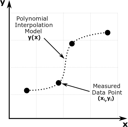
Figure 1: Interpolation of discrete data.

Once the user has input the two vectors of data (x and y, for instance), the polyfit() function can be used to interpolate the data to a polynomial function. The polyfit() function stores the coefficients of the polynomial in vector form, where they can later be used to generate the polynomial interpolation model. The polyval() function uses polynomial coefficients (the output of the polyfit() function) to find the interpolated value of y at a chosen value or vector of x.

For interpolation, the order of the polynomial must be exactly one less than the total number of data pairs. So for given data \(\left( \text{x}_{\text{1}},\text{y}_{\text{1}} \right)\text{,…,}\left( \text{x}_{\text{n}\text{+1}},\text{y}_{\text{n}\text{+1}} \right)\), the polynomial obtained would be of the form \(\text{y} = \text{a}_{\text{1}}\text{x}^{\text{n}} + \text{a}_{\text{2}}\text{x}^{\text{n} - \text{1}} + \text{…} + \text{a}_{\text{n}}\).

The polyfit() function is used to output the coefficients of the polynomial that passes through the data pairs. The output is stored as a vector \(\displaystyle{\lbrack a_1, \ a_2,...,a_n \rbrack}\). With these coefficients, the user can symbolically develop the interpolation function and if needed, conduct integration, differentiation, and plotting. Note that the first element corresponds to the coefficient of the highest power \(\left( x^n \right)\), while the last element corresponds to the constant of the polynomial model.

The polyval() function takes the output of the polyfit() function and uses it to evaluate the value of the polynomial interpolant at a given value (or a vector) of x. That is, polyval() substitutes values for x into the polynomial model. Then polyval() returns the corresponding values of y (the predictions) from the polynomial (see Example 1).

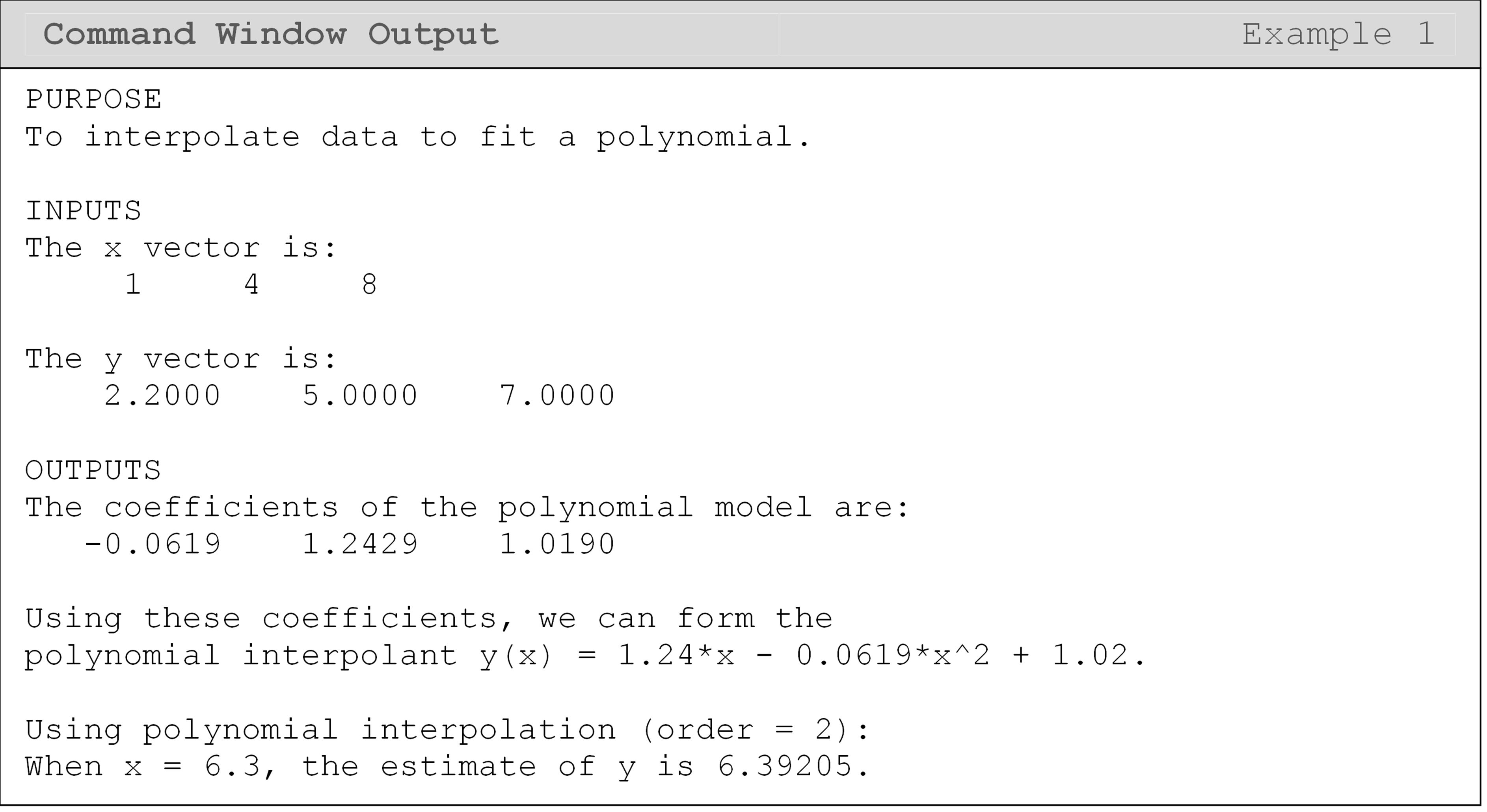
Example 1

Using a polynomial model, interpolate the (x, y) data pairs in Table A to a polynomial. Find the value of the interpolant at x = 4.5 and output it to the Command Window.

Table A: Data pairs for Example 1.

x	1.0	4.0	8.0
y	2.2	5.0	7.0

Solution

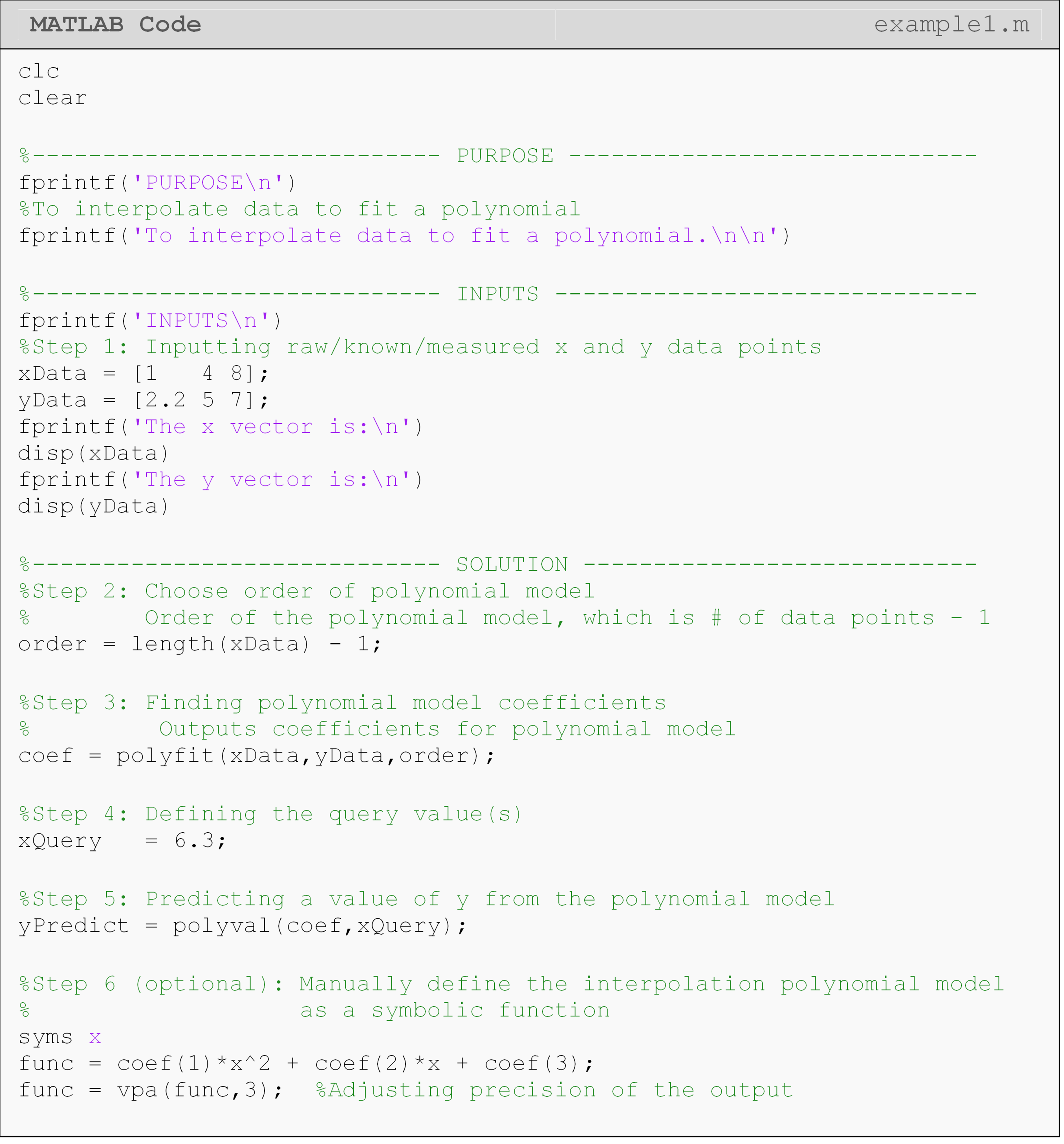
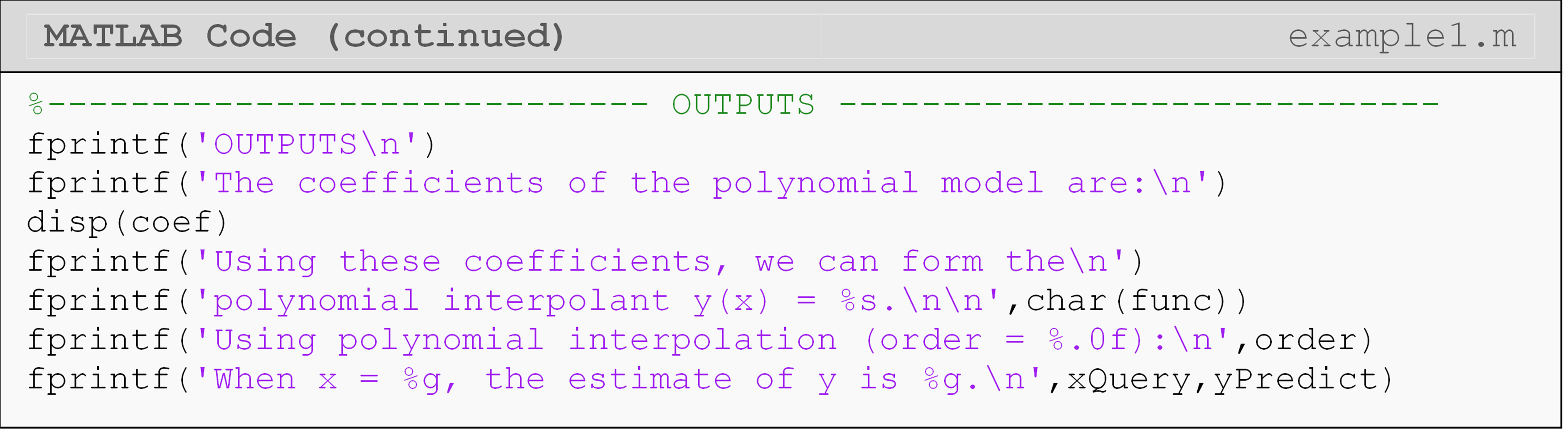
We “hardcoded” the polynomial expression in Example 1 for learning efficiency. This way, you can see how a symbolic function can be manually defined from its coefficients (the output of polyfit()). See Example 3 for a better method to do this without hardcoding: poly2sym().

What is spline interpolation?

Spline interpolation uses multiple “spline” (math) functions to fit the given data points (Figure 2). Taken as a whole, these splines form a piecewise continuous function: meaning the final model is made up of pieces or splines. Splines can be based on different models, but are commonly linear (\(f(x)=a_1x+a_2\)) or cubic (\(f(x)=a_1x^3+a_2x^2+a_3x+a_4\)) polynomial functions.

How do I conduct spline interpolation?

When compared to polynomial interpolation, using splines to interpolate the data can prove to be very beneficial in many circumstances. These splines are typically linear or cubic in form and can be implemented in MATLAB using the function interp1().

In some cases, especially with higher order polynomials, a polynomial interpolant can be a bad idea as it may give oscillatory behavior (Figure 4) for otherwise well-behaved smooth functions. When provided a large number of data points, spline interpolation is generally better suited.

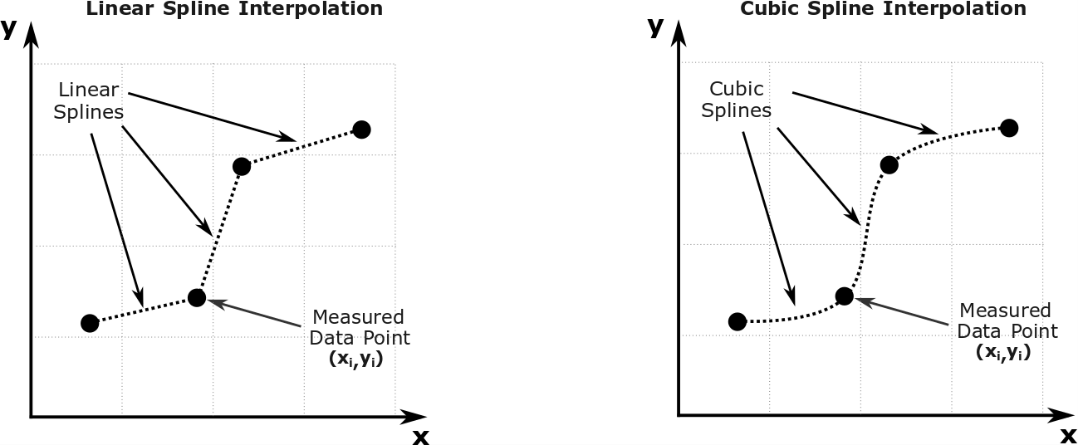
Figure 2: Spline interpolation of discrete data.

Often times when interpolating a data set, a linear spline model is sufficient. In such a case, each data point is connected to the next with a straight line (Figure 2). This technique is commonly used in interpolating data from thermodynamic steam tables. If this is not sufficient, a cubic spline is often used, which connects the data points with cubic functions (nonlinear lines as shown in Figure 2). The MATLAB function, interp1(), can be used to interpolate a data set using a specified model (including a linear or cubic-spline model). An example of the usage of this function is: interp1(xData, yData, xQuery, 'method').

The output of the interp1() function is a vector of the same size as the input vector of the x value(s). We call these input values “x query” values because they are the values of the independent variable at which we want to make predictions. For example, when x = 3, what is the value of y? Here, “x = 3” is the query value. Table 1 shows the common interpolation methods that can be used as the input for the interp1() function, and Example 2 shows the function in action.

Table 1: Common interpolation models to be used with the interp1() function.

Interpolation Method	Interpolation Model Generated
`'linear'`	Interpolates via straight lines between each consecutive point (default model).
`'spline'`	Connects each point with a cubic-spline interpolant. The first and second derivatives of the adjoining splines will be continuous.

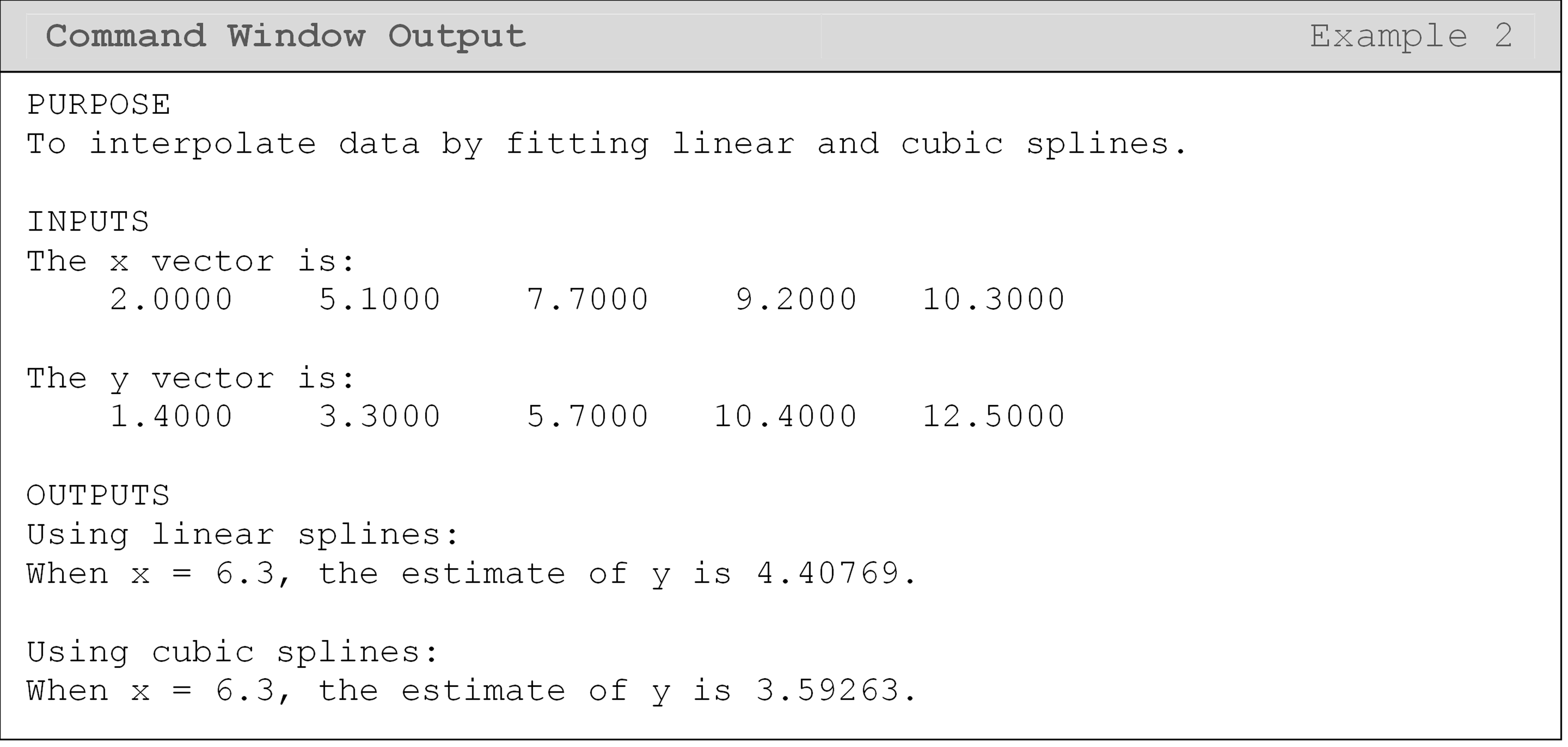
Example 2

Interpolate the (x,y) data pairs from Table B using linear and cubic spline interpolation. Output the predictions using fprintf() at x = 6.3.

Table B: Data pairs to be used for Example 2.

x	2.0	5.1	7.7	9.2	10.3
y	1.4	3.3	5.7	10.4	12.5

Solution

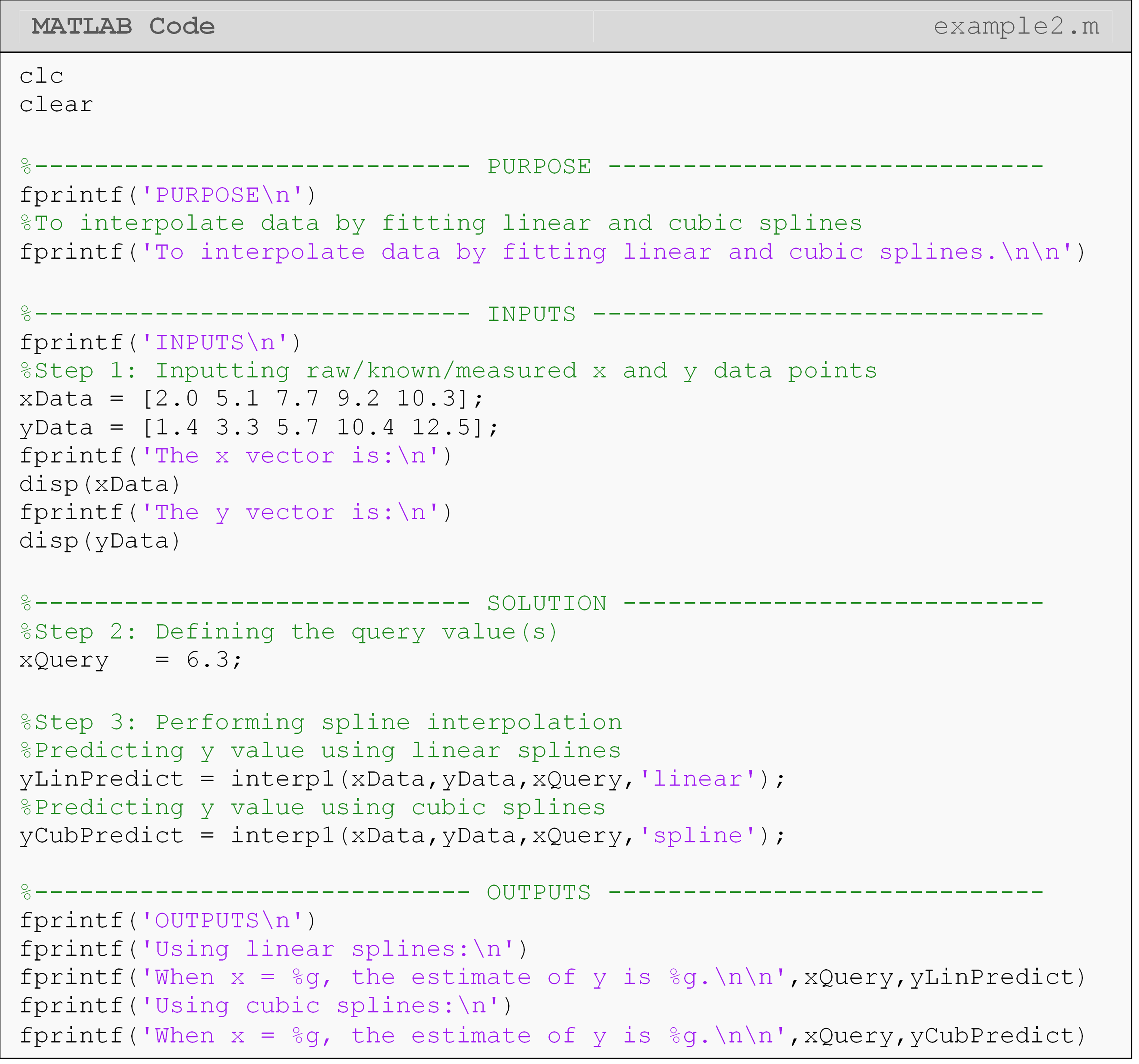
The Command Window output shows the predicted y values when x = 6.5. These values are fairly different from each other (3.593 for linear splines vs. 4.408 for cubic splines). In the next lesson (Lesson 4.8), you will be able to see more clearly why this is so when we plot the linear and cubic spline functions.

What is regression?

Finding a function that best fits the given data pairs is called regression. When conducting interpolation, all data pairs used must be on the developed curve. On the other hand, a regression curve is not constrained by this requirement. Using MATLAB to develop a regression curve is useful, especially for experimental data, or for developing simplified models.

Let us suppose someone gives you n data pairs:\((x_1,y_1),(x_2,y_2),...,(x_n,y_n)\), and you want to develop a relationship between the two variables. A simple example is that of measuring stress vs. strain data for a steel specimen under loads lower than the yield point. We expect that the relationship between stress and strain is a straight line. However, because of material imperfections and inaccuracies in data collection, we are not going to get all the data points on a straight line. So, we do the next best thing – draw a straight line that minimizes the sum of the square of the difference between the observed and predicted values (Figure 3). How that is done is a subject for a course in statistics or numerical methods.

In this part of the lesson, we will just concentrate on how to use MATLAB to regress data to polynomials. Although there is a mathematical/statistical difference between polynomial interpolation and regression, there is no explicit difference in MATLAB syntax between an interpolation and regression polynomial. Therefore, you should choose the curve fitting method that makes the most sense or gives the best results for your problem.

One of the challenges when fitting some models to a data set is the tendency to overfit the data. We will not go into great detail in this lesson, but we want to alert you to this important and common problem. When performing polynomial regression, you should try to choose an order for the polynomial that does not overfit the data.

MATLAB will often display a warning that your polynomial is “badly conditioned” when you are overfitting. Another sign of overfitting is when you have large deviations from your expected curve (see Figure 4). For example, if you had position and time data from an accelerating car, you would not expect to see something like Figure 4 where there is a large deviation from the expected path. Therefore, thinking critically about your results is essential!

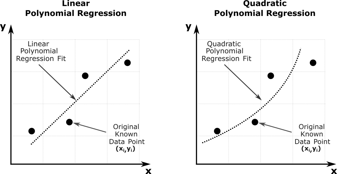
Figure 3: Regression of n data points to best fit a given order polynomial.

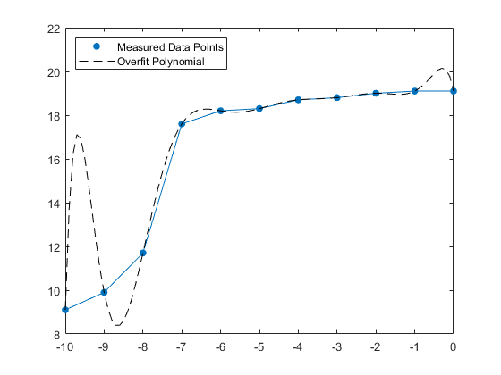
Figure 4: An example of overfitting on position and time data from an accelerating car (code not shown).

How do I do regression in MATLAB?

Similar to interpolation, the first step of making a regression model is to determine the type of function that best fits the data pairs. This lesson will focus on the polynomial regression model, although many other regression models may be used. These other models include exponential, power, and saturation growth models.

To do polynomial regression, you need the following two inputs:

Data pairs (x, y)
Order of the polynomial of regression, m

For regression, the order of the polynomial chosen must be less than (total number of data pairs minus one). So for given data pairs \((x_1,y_1),...,(x_n,y_n)\), the polynomial obtained would be of the form \(\displaystyle{y=a_1x^m+a_2x^{m-1}+...+a_m}, \ 1\leq m \leq n-2\). Note that for \(\text{m} = \text{n} - 1\) the regression polynomial would be an interpolating polynomial.

The polyfit() function is used to output the coefficients of the regression polynomial. The output is stored as a vector \(\displaystyle{\lbrack a_1,a_2,...,a_m\rbrack}\). With these coefficients, the user can symbolically develop the regression function and if needed, conduct integration, differentiation, and plotting. Note that the first element corresponds to the coefficient of the highest power (x^m), while the last element corresponds to the constant of the polynomial model.

The function polyval() can be used again for the same purpose as shown in Example 1. In Example 3, it will take the coefficients of a polynomial and x query value(s) as inputs and return the predicted value for y, which it obtains from the regression polynomial.

Example 3

Using MATLAB, regress the given (x, y) data pairs from Table C to a linear and quadratic regression model, and predict the value of y when x is \(\displaystyle{(-300, \ -100, \ 20, \ 125)}\) using both models. Output the predictions and the regression models using fprintf() or disp().

x	340	280	200	120	40	40	80
y	2.45	3.33	4.30	5.09	5.72	6.24	6.47

Table C: Data pairs to be used for Example 3.

Solution

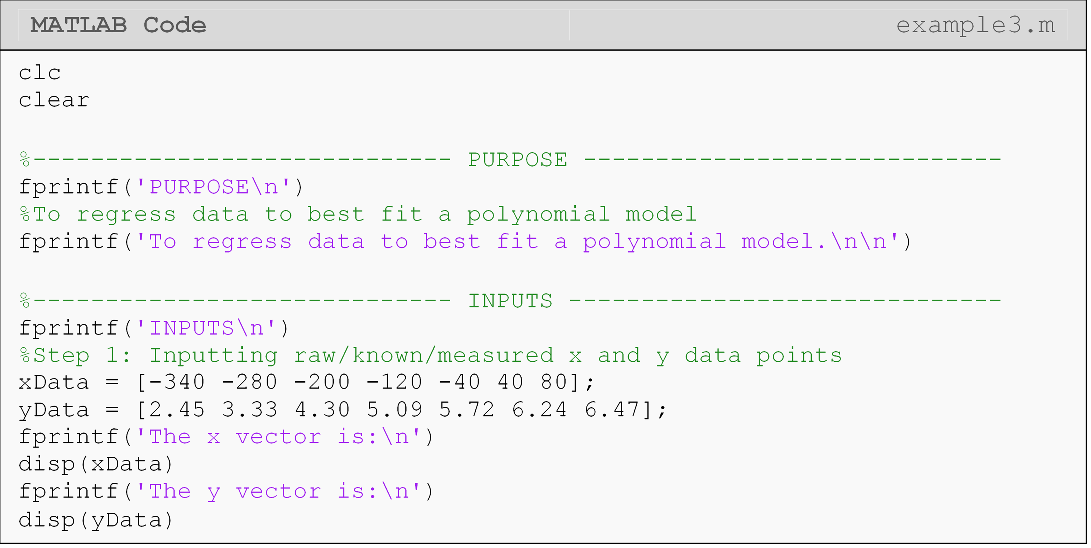
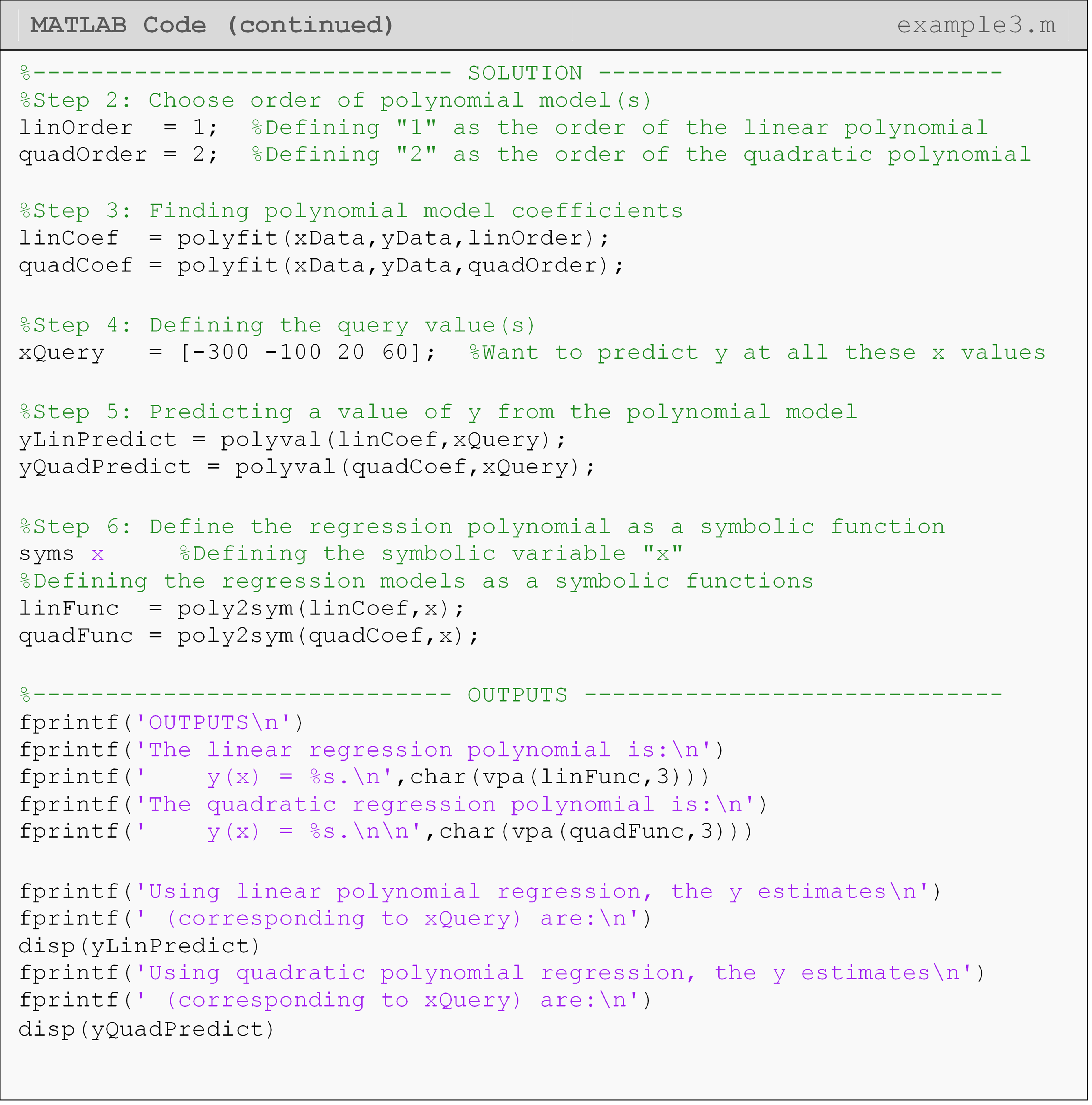
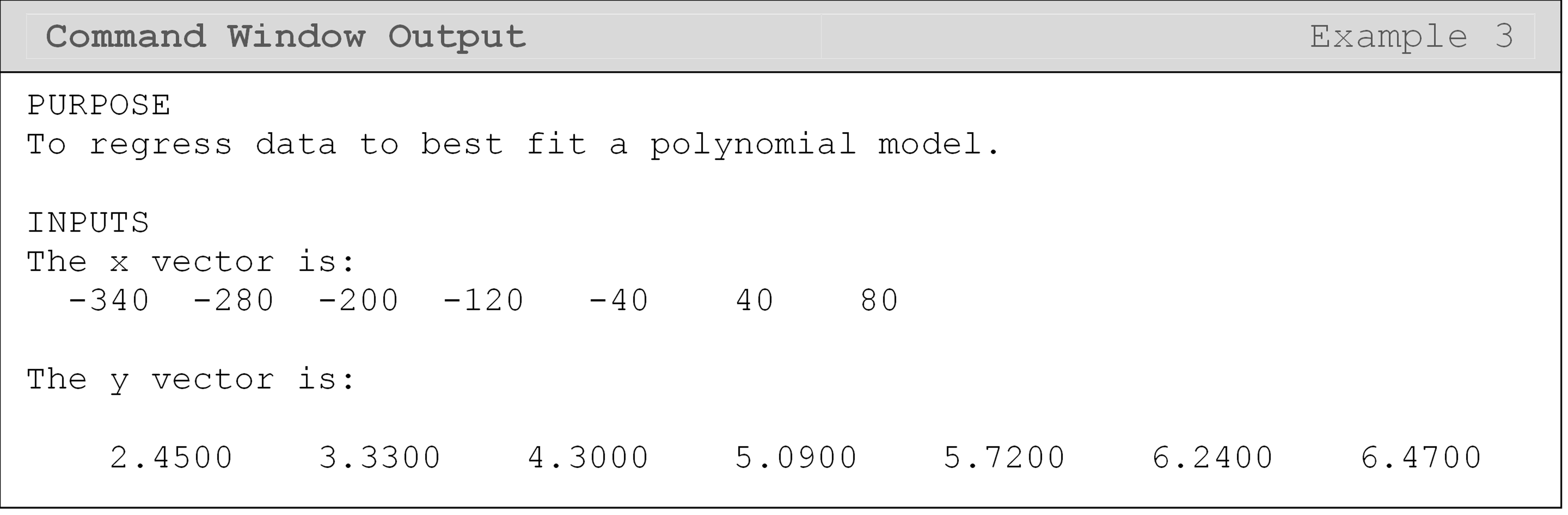
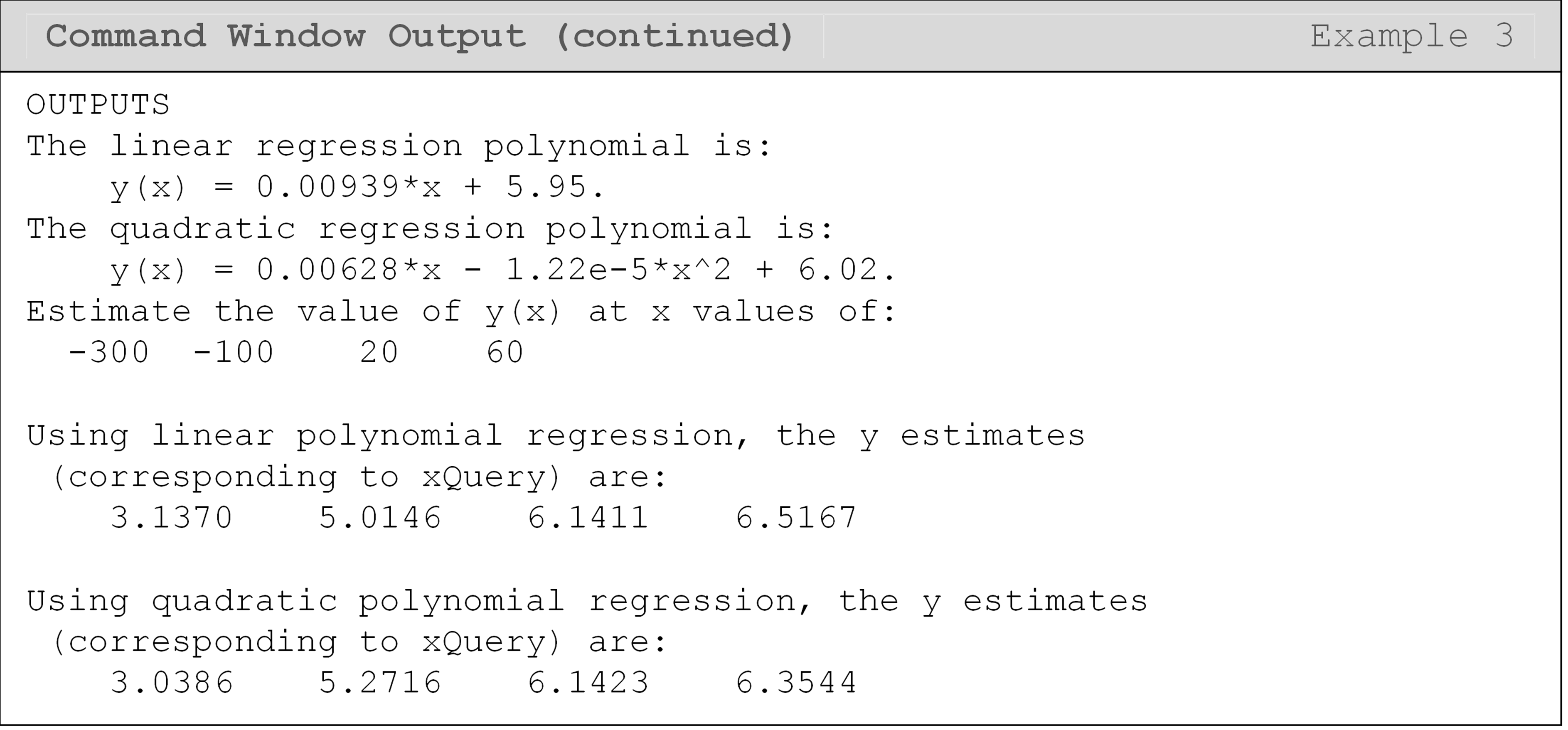
In Example 3, since we are inputting a vector of values to polyval() (using the variable xQuery), it will return a vector of predictions to us, which can be seen in the Command Window output. Remembering the inputs and outputs of these curve fitting functions is essential to proper implementation.

Lesson Summary of New Syntax and Programming Tools

Task	Syntax	Example Usage
Polynomial interpolation	`polyfit()`	`polyfit(x,y,order)`
Polynomial regression	`polyfit()`	`polyfit(x,y,order)`
Spline interpolation	`interp1()`	`interp1(x,y,xQuery,'method')`
Convert polynomial coefficients to symbolic function form	`poly2sym()`	`poly2sym(coef,x)`

Multiple Choice Quiz

(1). The MATLAB function used to find the coefficients of a polynomial interpolation or regression model for given data pairs is

(a) polyfit()

(b) polyval()

(d) interceof()

(2). The result of the curve fitting procedure completed in the following program is

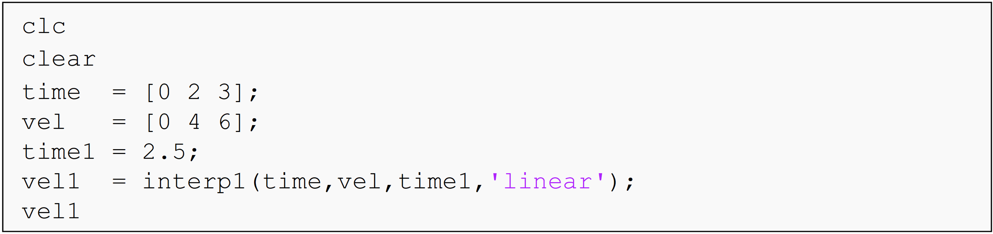
(a) polynomial interpolation

(b) spline interpolation

(d) None of the above

(3). The output of the last line is

(a) 2.5

(b) 5.0

(d) 10.0

(4). Complete the code to output the regression model as a symbolic function.

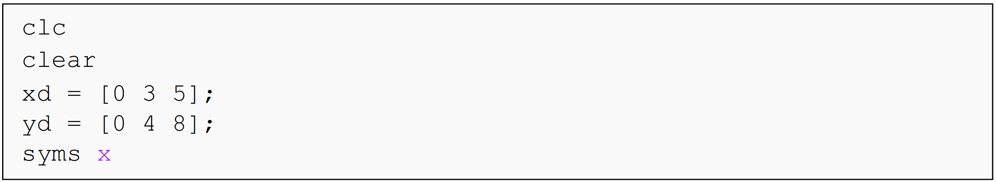
(a) coef = polyfit(xd,yd,1);y = coef(2)*x + coef(1)

(b) coef = polyfit(yd,xd,1);y = coef(2)*x + coef(1)

(d) coef = polyfit(yd,xd,1);y = coef(1)*x + coef(2)

(5). The function that uses previously found coefficients of a polynomial interpolant as an input to calculate the value of the function at a given point is

(a) polyfit()

(b) polyval()

(d) intereval()

Problem Set

(1). Given are \((x,y)\) data pairs in Table A.

Table A: Data pairs for Exercise 1.

x	1.4	2.3	5.0	7.5
y	3.2	1.7	6.1	3.8

Complete the following.

(a) Interpolate the data using a polynomial interpolant. Find the value of y when x = 4.75.

(b) Interpolate the data using linear spline interpolation. Find the value of y when x = 4.75.

(2). The upward velocity of a rocket is given as a function of time in Table B.

Table B: Upward rocket velocity at a given time.

*t (s)*	0	10	15	20	22.5	30
*v(t) m/s*	0	227.04	362.78	517.35	602.97	901.67

Using MATLAB, complete the following.

(a) Using a polynomial interpolant, find velocity as a function of time.

(b) Find the velocity at t = 16 s.

(3). A curve needs to be fit through the seven points given in Table C to fabricate the cam. The geometry of a cam is given in Figure A.

Each point on the cam shown in Figure A is measured from the center of the input shaft. Table C shows the x and y measurement (inches) of each point on the camshaft.

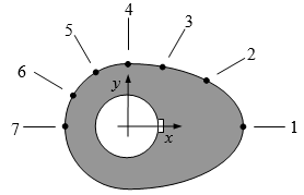
Figure A: Schematic of cam profile

Table C: Geometry of the cam corresponding to Figure A.

Point	x (in)	y (in)
1	2.20	0.00
2	1.28	0.88
3	0.66	1.14
4	0.00	1.20
5	-0.60	1.04
6	-1.04	0.60
7	-1.20	0.00

Using MATLAB, find a smooth curve that passes through all seven data points of the cam. Output this model to the Command Window.

(4). Using MATLAB, regress the following (x, y) data pairs (Table D) to a linear polynomial and predict the value of y when \(x= 55,20, - 10.\)

Table D: Data pairs (x, y) for Exercise 1.

x	y
325	2.6
265	3.8
185	4.8
105	5.0
25	5.72
– 55	6.4
– 70	7.0

Use the fprintf() and/or the disp() functions to output the regression model and the predictions to the Command Window.

(5). To simplify a model for a diode, it is approximated by a forward bias model consisting of DC voltage, \(\text{V}_{\text{d}}\), and resistor, \(\text{R}_{\text{d}}\). Below is the collected data of current vs. voltage for a small signal (Table E).

Table E: Current versus voltage for a small signal.

V (volts)	I (amps)
0.6	0.01
0.7	0.05
0.8	0.20
0.9	0.70
1.0	2.00
1.1	4.00

Regress the data in Table E to a linear model of the voltage as a function of current. Approximate the voltage when 0.35 amps of current is applied to the diode and output this result using fprintf().

(6). To find contraction of a steel cylinder, one needs to regress the thermal expansion coefficient data to temperature. The data is given below in Table F.

Table F: The thermal expansion coefficient at given temperatures

Temperature, T \((^\circ F)\)	Coefficient of thermal expansion, \(\alpha\) \((\text{in/in/}^\circ F)\)
80	\[6.47 \times 10^{- 6}\]
40	\[6.24 \times 10^{- 6}\]
– 40	\[5.72 \times 10^{- 6}\]
– 120	\[5.09 \times 10^{- 6}\]
– 200	\[4.30 \times 10^{- 6}\]
– 280	\[3.33 \times 10^{- 6}\]
– 340	\[2.45 \times 10^{- 6}\]

Find the coefficient of thermal expansion when the temperature is \(-150^\circ F\) using

(a) linear polynomial regression,

(b) quadratic polynomial regression, and