Module 4: MATH AND DATA ANALYSIS
Learning Objectives
After reading this lesson, you should be able to:
perform linear algebra operations on matrices,
solve systems of equations with MATLAB.
Note that the basics of matrices and vectors in MATLAB were covered in Lesson 2.6. We do not repeat them here.
What is linear algebra?
Linear algebra is the set of rules and operations dealing with equations that contain matrices (for the scope of this book). In this lesson, we review the basics of linear algebra: how to add, subtract, and multiply matrices and vectors and a few other common operations. However, our main focus will be on MATLAB. It is essential to learn these basics since vectors and matrices are very common in programming for a variety of applications. We have included a primer on linear algebra in Appendix A in case you need further practice with the fundamentals of linear algebra. If you do not know how to do the operations discussed in this lesson on paper, be sure to get up to speed on them. Doing so will save you time in the long run as programming them requires a fundamental understanding in most cases.
 Important Note: Remember
a vector is a special type of matrix: a single column or single row
matrix. Therefore, everything said about matrices in this lesson
includes vectors as well.
Important Note: Remember
a vector is a special type of matrix: a single column or single row
matrix. Therefore, everything said about matrices in this lesson
includes vectors as well.
How do I add and subtract matrices?
To add or subtract two matrices, the two matrices have to be the same dimension (both matrices need to have the same number of rows and columns). Figure 1 shows an example of matrix addition, where two rectangular matrices of size \(3 \times 2\) are added together. Example 1 demonstrates how to perform matrix addition in MATLAB.
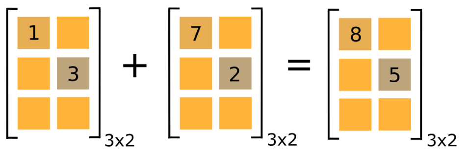
Figure 1: Example of matrix addition. Only the addition of the two
elements is shown in this visual example.
Can I use math functions like sin() on matrices?
As mentioned in previous lessons, to find the sine of each element in
a matrix, just give MATLAB the matrix as an input. That is, if \([A]\) is
your matrix, sin(A) will return a matrix of the sine of each element
in \([A]\). The same is true for all the trigonometric, exponential, and
logarithmic functions. As you can see in Example 1, the same
mathematical functions (sin(), log(), exp(), etc.) can be used on
matrices with no change in syntax.
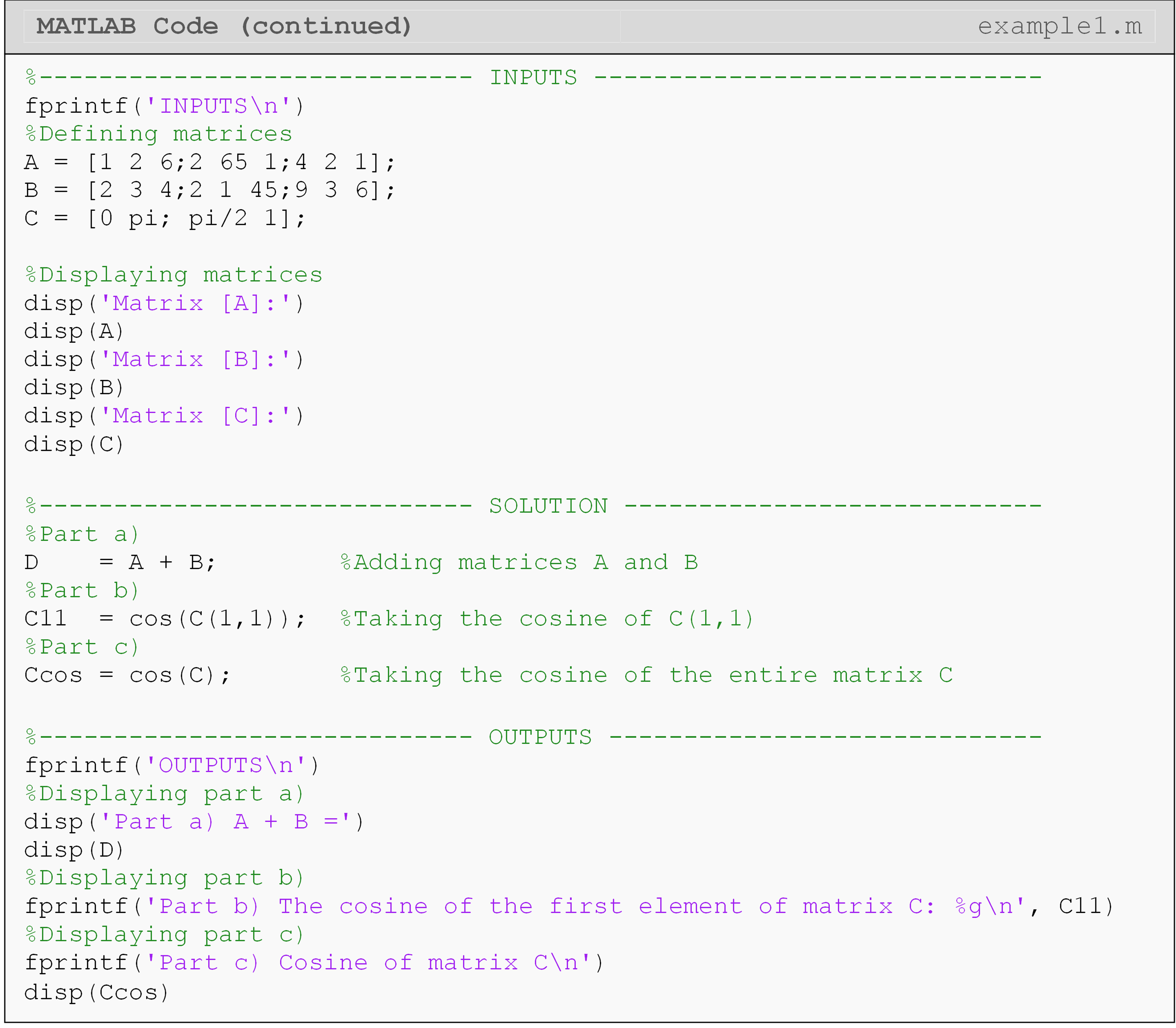
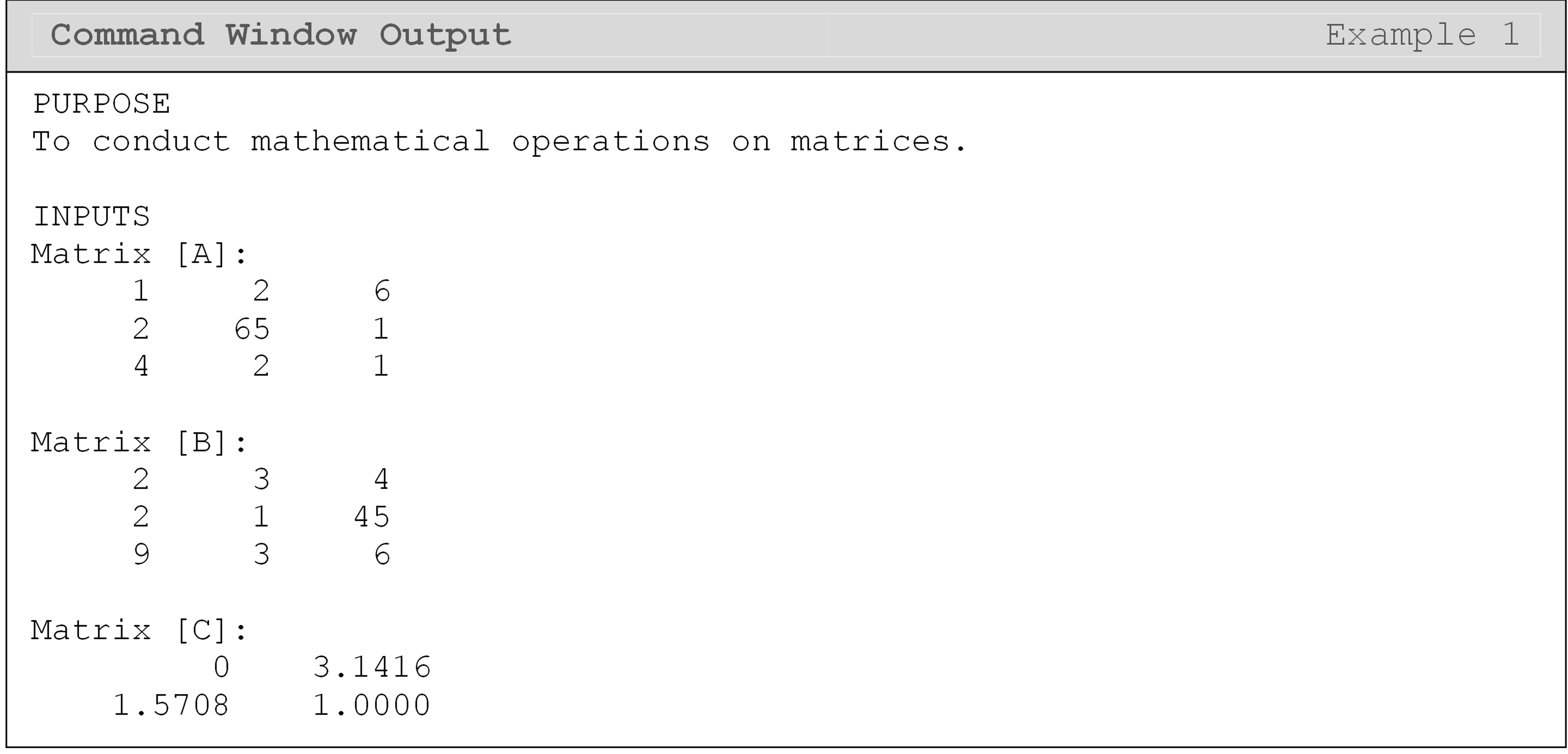
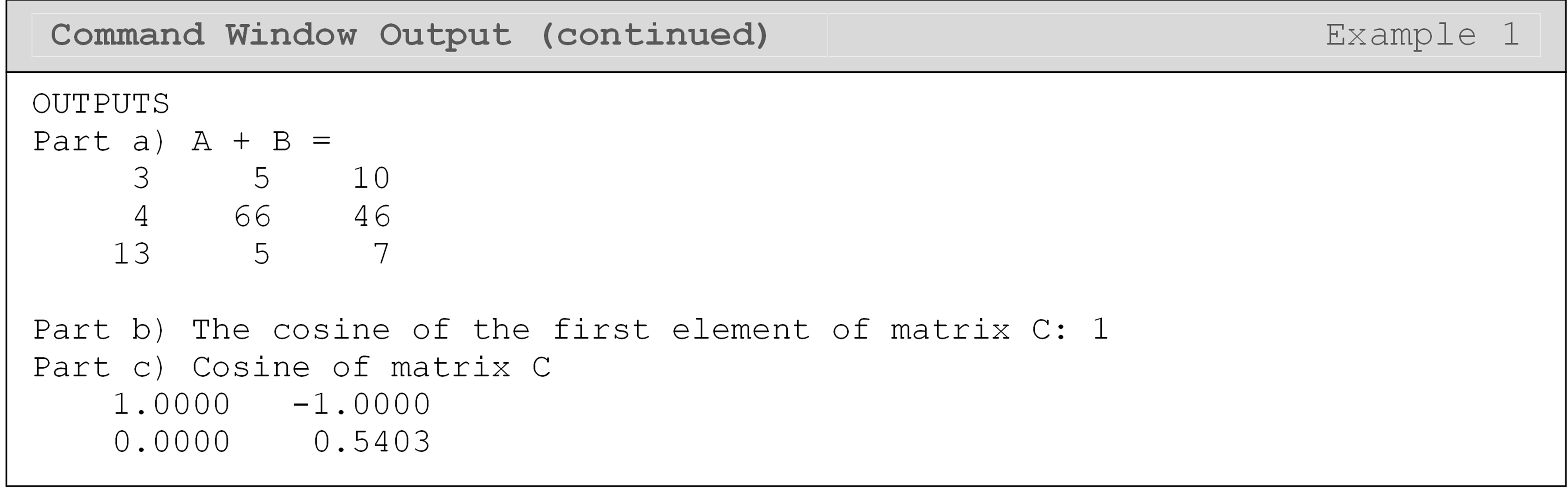
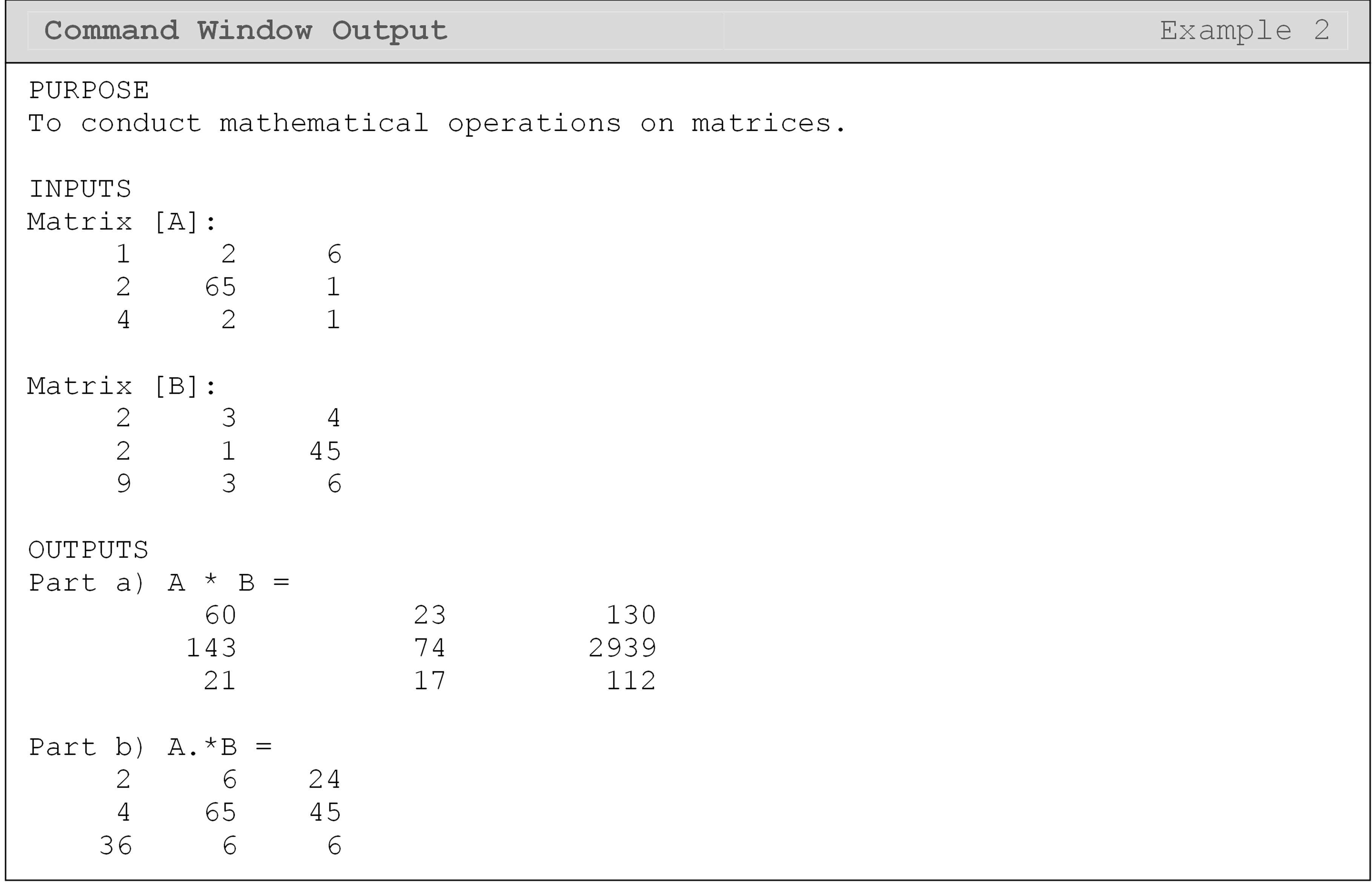
Example 1
Input the following two matrices, \([A]\) and \([B]\), into a new m-file.
\(\lbrack A\rbrack = \begin{bmatrix} 1 & 2 & 6 \\ 2 & 65 & 1 \\ 4 & 2 & 1 \\ \end{bmatrix}\) \(\lbrack B\rbrack = \begin{bmatrix} 2 & 3 & 4 \\ 2 & 1 & 45 \\ 9 & 3 & 6 \\ \end{bmatrix}\) \(\text{[}\text{C}\text{]} = \ \begin{bmatrix} \text{0} & \pi \\ \displaystyle\frac{\pi}{\text{2}} & \text{1} \\ \end{bmatrix}\)
Conduct the following operations:
Add the two matrices \([A]\) and \([B]\)
Find the cosine of C(1,1)
Find the cosine of all the elements in \([C]\)
Solution
How do I perform matrix multiplication?
Unlike addition and subtraction, matrix multiplication is not simply the product of each set of elements: e.g., A(1,1)*B(1,1). You do not absolutely need to understand how to do this by hand, but you must understand two resulting facts:
Inner dimensions of a matrix product must be equal: \(\text{A}_{\text{m} \times \text{n}} \times \text{B}_{\text{n} \times \text{p}}\) . That is, the number of columns of the first matrix has to be equal to the number of rows of the second matrix.
Matrix products are not commutative. That is, in general, the order of the two matrices matters \(([A]\text{*}[B]\text{ does not equal }[B]\text{*}[A])\).
An example of matrix multiplication can be seen in Figure 3, while a full MATLAB code of multiplying two matrices together is shown in Example 3.
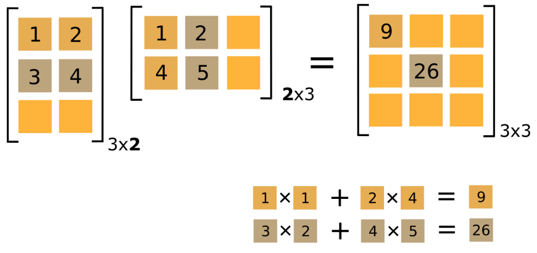
Figure 3: An example of matrix multiplication. Only two calculated
elements are shown.
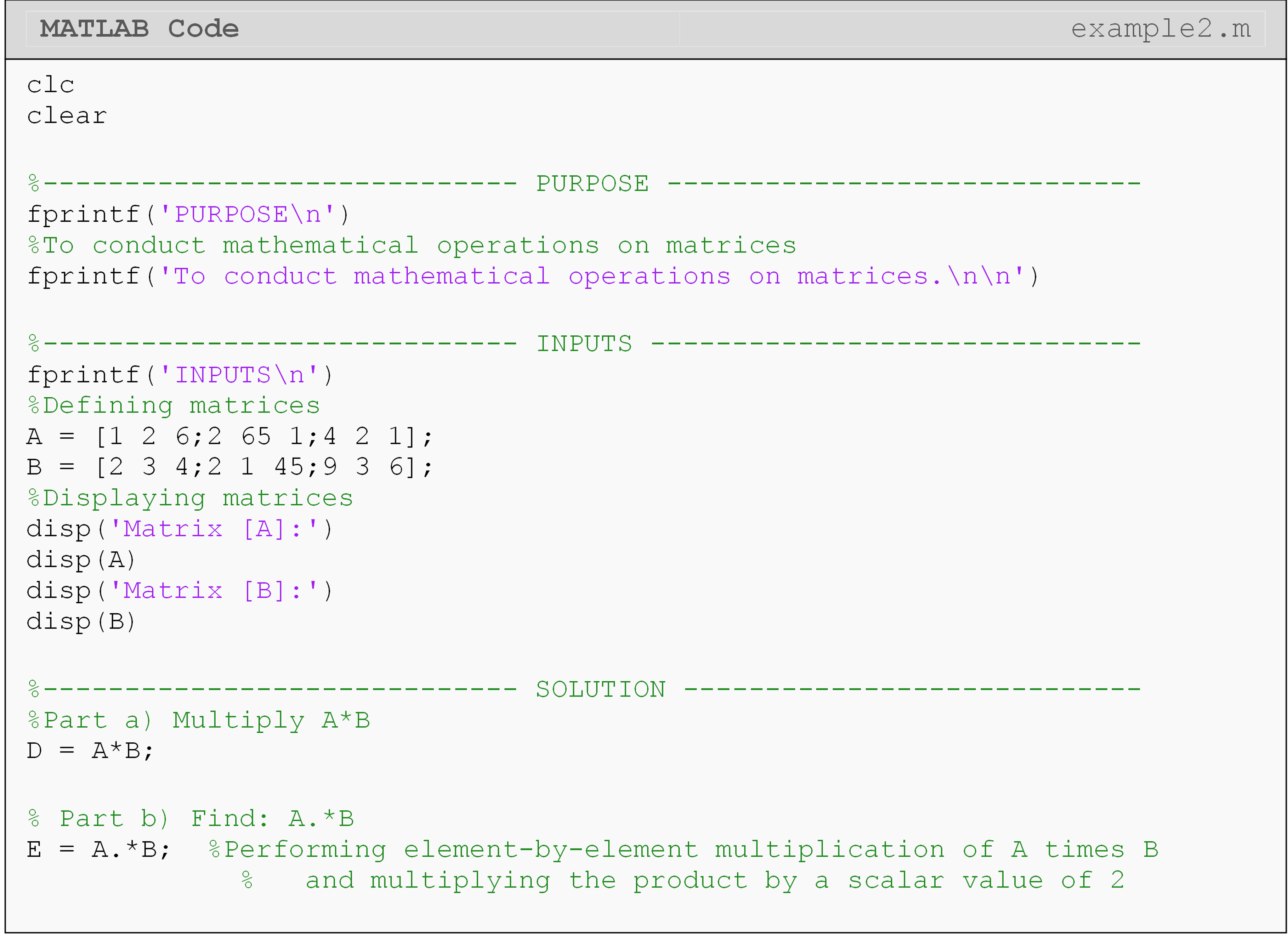
What is the difference between matrix and array operations?
Array operations performed element-by-element operations to matrices
(and vectors). Matrix operations are traditional matrix algebra
operations as outlined in the previous sections of this lesson and in
Appendix A. Array operations have a dot next to the math operator. For
example, A*B would perform a matrix multiplication of matrix A and
B. However, matrix A.*B would multiply each element of A and B
together (not the same answer as you can see in Example 2!), and
requires the matrices to have equal dimensions.
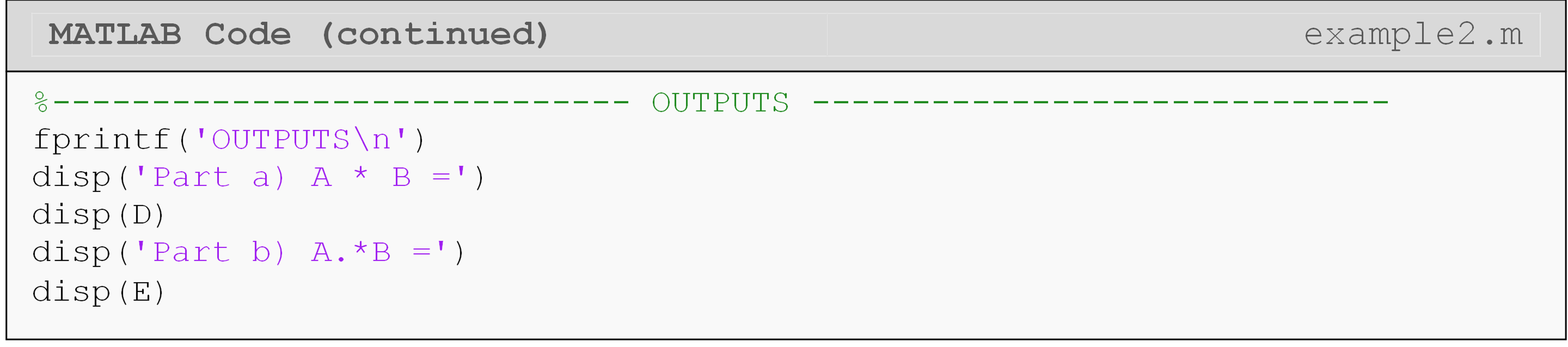
Example 2
Input the following two matrices, \([A]\) and \([B]\), into a new m-file.
\(\lbrack A\rbrack = \begin{bmatrix} 1 & 2 & 6 \\ 2 & 65 & 1 \\ 4 & 2 & 1 \\ \end{bmatrix}\) \(\lbrack B\rbrack = \begin{bmatrix} 2 & 3 & 4 \\ 2 & 1 & 45 \\ 9 & 3 & 6 \\ \end{bmatrix}\)
Conduct the following operations:
Multiply matrix \([A]\) by \([B]\).
Conduct element to element multiplication of the two matrices \([A]\) and \([B]\).
Solution
As you can see, as long as the rules for matrix operations are followed (as given in Appendix A), adding, subtracting and multiplying matrices requires no different symbols than from what we are used to for simple scalar operations. However, recall that matrix division is undefined. To solve this problem, the MATLAB programmers introduced a function that finds the inverse of a square matrix.
Table 1: Several commonly used matrix functions and operators. The inputs listed are the matrices \([A]\) and \([B]\) (where applicable).
| Operation | Syntax | Function | Rules |
|---|---|---|---|
| Addition | A+B |
Adds two matrices. | All dimensions must be equal. |
| Subtraction | A-B |
Subtracts two matrices. | All dimensions must be equal. |
| Multiplication (matrix) | A*B |
Multiplies two matrices. | Inner dimensions must be equal. |
| Multiplication (by scalar) | 5*B |
A scalar times a matrix. | Multiplies each element of the matrix by the scalar. No array operator needed. |
| Array operations | . |
Conduct a specified element to element operation (see usage example below). | Depends on usage. |
| Multiplication (array) | A.*B |
Multiplies two matrices element-by-element. | Matrices must have equal dimensions. Array operator required. |
| Matrix inverse | inv(A) |
Outputs the inverse of a matrix. | Must be a square matrix. |
| Exponent (matrix) | A^2 |
Equivalent to [A]*[A] | Must be a square matrix. |
| Exponent (array) | A.^2 |
Raise each element, A(i,j), to power | Can be any size. |
Notice that in Table 1, there is no function to conduct matrix division. This is because matrix division is not defined for matrices. However, one may also use the arithmetic division operator with the array (.) operator to conduct element-by-element division of one matrix by another.
How do I take the inverse of a matrix?
Recall that multiplying a single number (scalar) by its inverse will
give a product equal to one (e.g.,
\(\text{5} \times \text{5}^{- \text{1}} = \text{1}\)). Similarly, for
matrices, multiplying a matrix by its inverse will yield the identity
matrix: all diagonal matrix elements are equal to “one” and all
non-diagonal elements are zero. An example of an identity matrix is
shown in Figure 3. In MATLAB, the inverse of a square matrix can be
found using the function
inv().
The inverse of a matrix is a key concept in linear algebra, so it is
important to understand it on a conceptual basis even for programming.
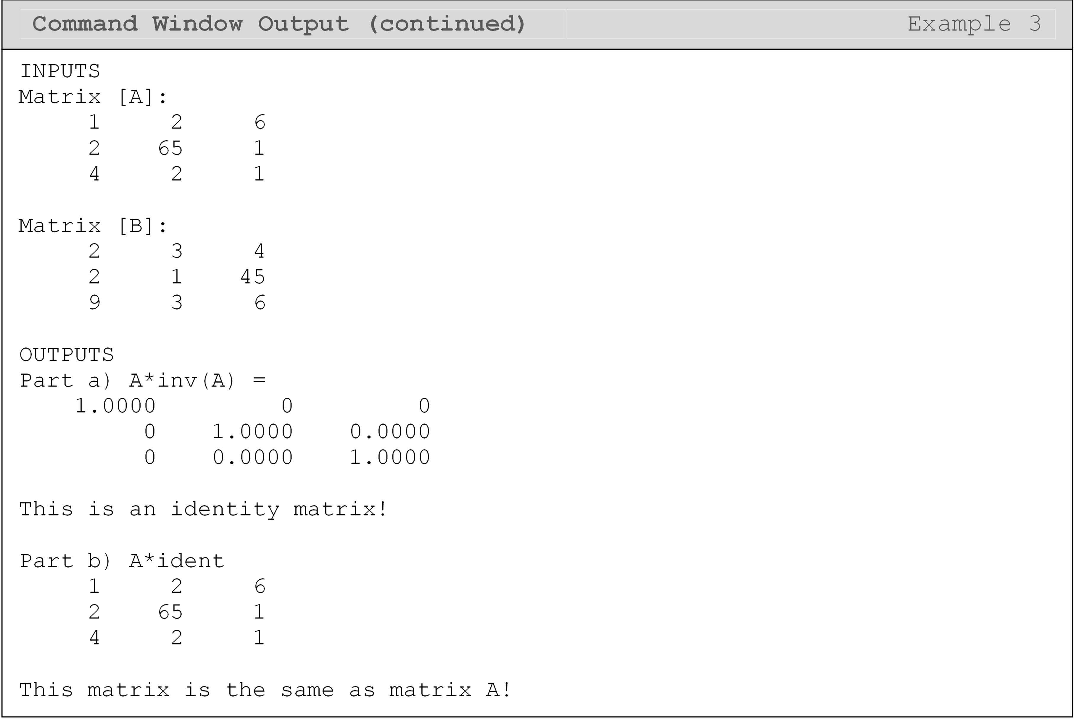
Example 3
Input the following two matrices, \([A]\) and \([B]\) into an m-file.
\(\lbrack A\rbrack = \begin{bmatrix} 1 & 2 & 6 \\ 2 & 65 & 1 \\ 4 & 2 & 1 \\ \end{bmatrix}\) \(\lbrack B\rbrack = \begin{bmatrix} 2 & 3 & 4 \\ 2 & 1 & 45 \\ 9 & 3 & 6 \\ \end{bmatrix}\)
Conduct the following operations:
Find the inverse of matrix \([A]\), naming it
invA. Now, multiply matrix \([A]\) byinvAand examine the resulting matrix.Find the size of matrix \([A]\) and develop an identity matrix of this size, naming it `ID. Multiply matrix \([A]\) by
IDand examine the resulting matrix.
Solution
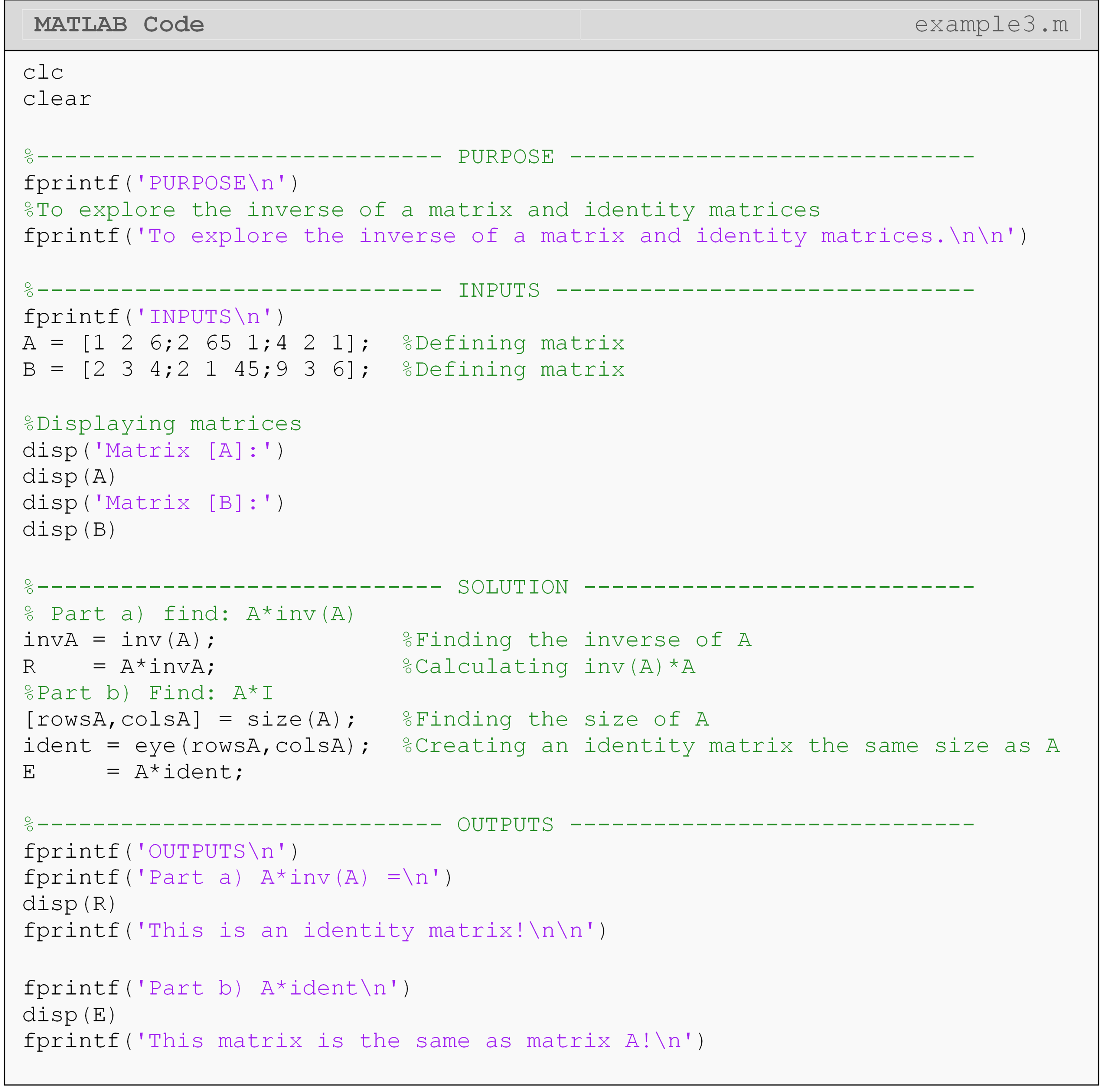
Examining the output of part (a) shows an identity matrix - this is what should be expected. In part (b) of Example 3, an identity matrix is multiplied to matrix \([A]\), and the resulting matrix is the same as matrix \([A]\). This is also in line with our expectations.
Can MATLAB do advanced matrix and vector operations?
There are a significant number of matrix operations available in MATLAB as predefined functions, and to cover them all would be out of the scope of this book. A few more common functions are shown in Table 2, and their usage is shown in Example 4. If you do not see the matrix operation you are interested in, try searching for the operation in MATLAB Help.
In Table 2, the functions to conduct a vector dot/cross product can be
modified to work with matrices. To do this operation, an additional
input to the function is required (adding the dimension after the listed
inputs). Use the MATLAB help menu and search the function name for more
details (e.g., >>doc max).
The norm() function has several norm types to choose from. For
example, Type 1 (i.e., norm(A,1)) is the largest column sum:
\(\left\|A\right\|_1 = \underset{\text{j}}{\text{max}} \left(\displaystyle\sum_{i=1}^{m}A_{ij}\right),j = 1,...,n\)
of an \(m \times n\) matrix.
The sort() function can also be modified from what is shown in Table 2
to numerically sort a vector from the largest number to the smallest by
using the inputs sort(A,'descend'). If the sort() function is used
as shown in Table 2, it will default to sort a matrix from the smallest
element to the largest element (in ascending order).
Table 2: Commonly used matrix functions. The input(s) to the listed functions is/are a matrix or vector\([A]\) and \([B]\) (where applicable).
| Task | Syntax | Explanation |
|---|---|---|
| Vector dot product | dot(A,B) |
Outputs the dot product of two vectors of equal length. |
| Vector cross product | cross(A,B) |
Outputs the cross product of two vectors of equal length. |
| Matrix transpose | A' |
Finds the transpose of a matrix. |
| Matrix Transpose | transpose(A) |
Finds the transpose of a matrix. |
| Smallest element | min(A) |
Outputs the smallest element in a vector. |
| Largest element | max(A) |
Outputs the largest element in a vector. |
| Sort an array | sort(A) |
Sorts a vector from least to greatest. |
| Matrix determinant | det(A) |
Outputs the scalar determinant of a square matrix. |
| Norm of a matrix | norm(A,p) |
Finds the norm of a matrix. |
| Trace of a matrix | trace(A) |
Outputs the scalar value of the trace of a matrix |
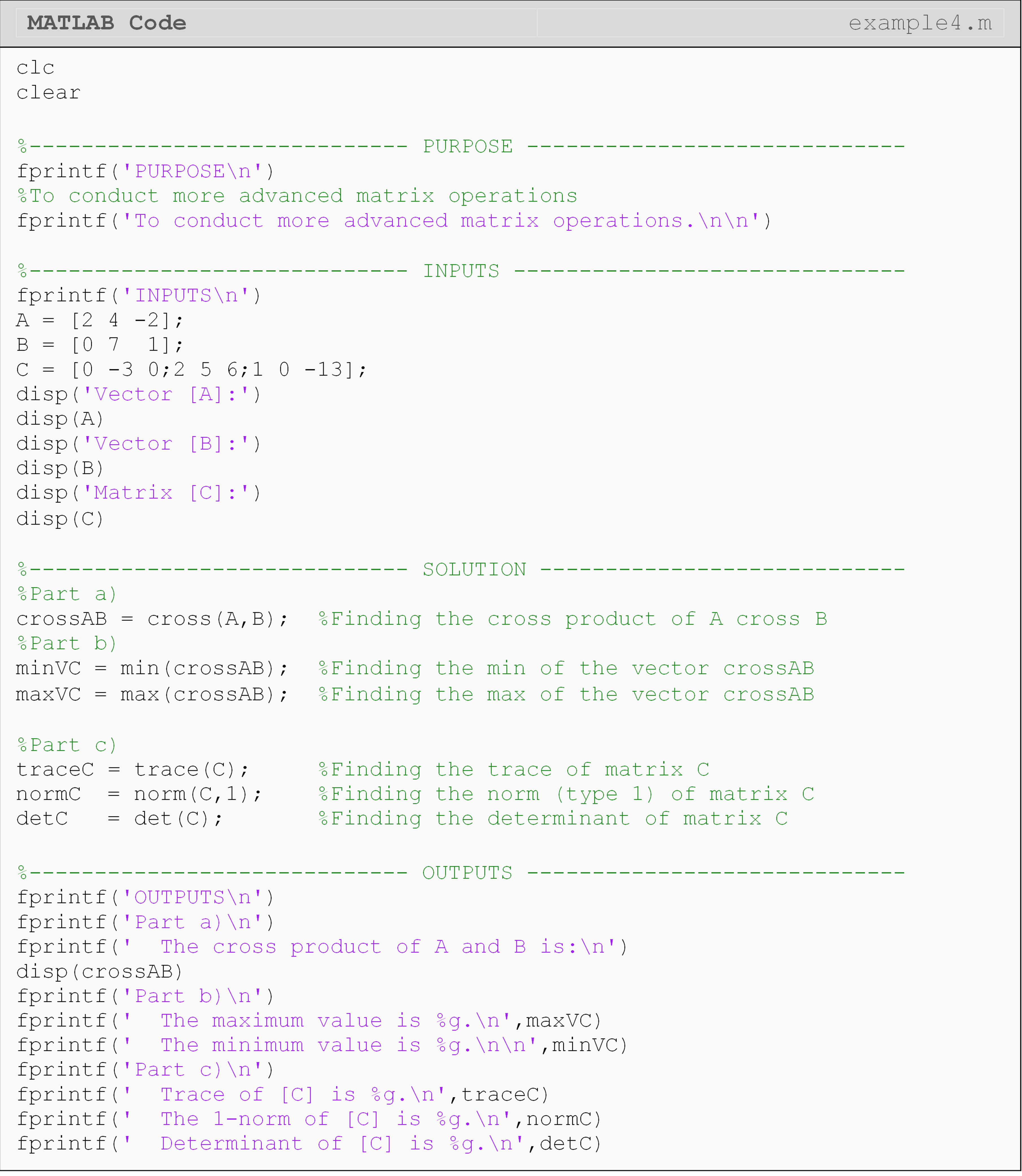
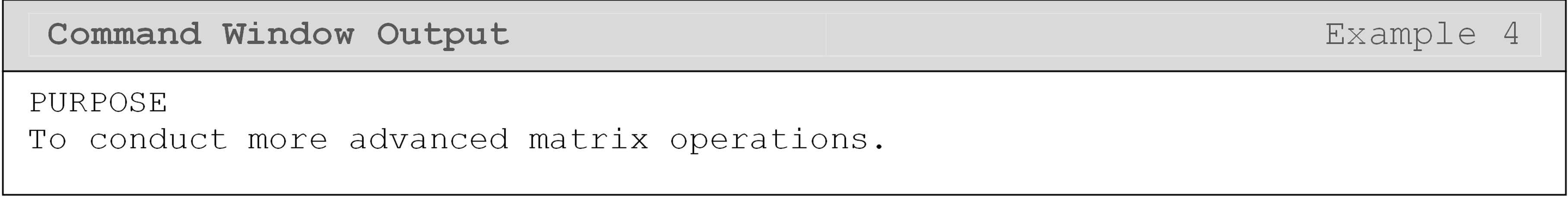
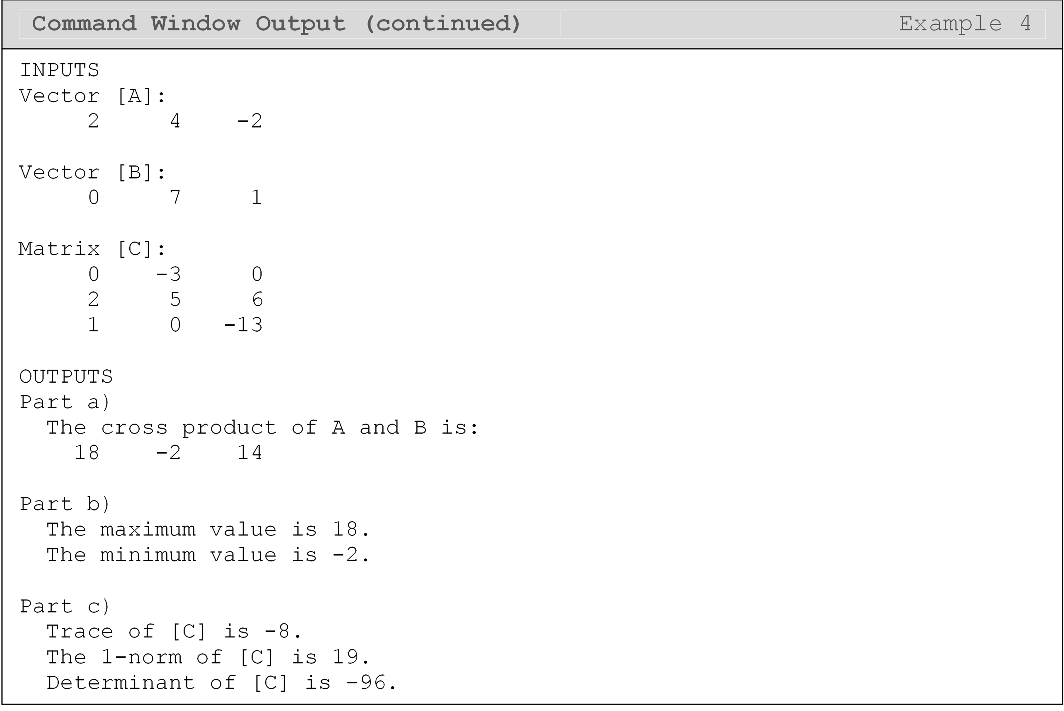
Example 4
Input the following two vectors, \([A]\) and \([B]\), and the matrix \([C]\) into a new m-file.
\[[A] = \begin{bmatrix} 2 & 4 & -2 \\ \end{bmatrix} \\{[B] = \begin{bmatrix} 0 & 7 & 1 \\ \end{bmatrix}} \\{[C] = \begin{bmatrix} 0 & -3 & 0 \\ 2 & 5 & 6 \\ 1 & 0 & -13 \\ \end{bmatrix}}\]
Using the functions listed in Table 2, complete the following:
Find the vector cross product of vectors \([A]\) and \([B]\), and name this new vector
crossAB.Find the value of the maximum and minimum element of vector
crossABfrom part (a).Find the numeric values of the trace, norm (maximum column sum), and determinant of matrix \([C]\).
Solution
How can I solve systems of equations with MATLAB?
One of the ways we can use MATLAB to harness the power of the computer is by it solving large systems of equations for us. A set of three equations and three unknowns may not be terribly hard to solve by hand, but there are many applications where that number is in the thousands.
To cut down on algebraic manipulation, matrices are commonly used to solve linear systems of equations. As outlined in Appendix A, to solve any linear system of equations a programmer must have (1) the coefficient matrix \(A\), (2) solution or unknown vector \(x\), and (3) the right-hand side vector \(C\). These three vectors/matrices are related in the following form \([A] \cdot [x] = [C]\). Examples 5 and 6 demonstrate this process in MATLAB.
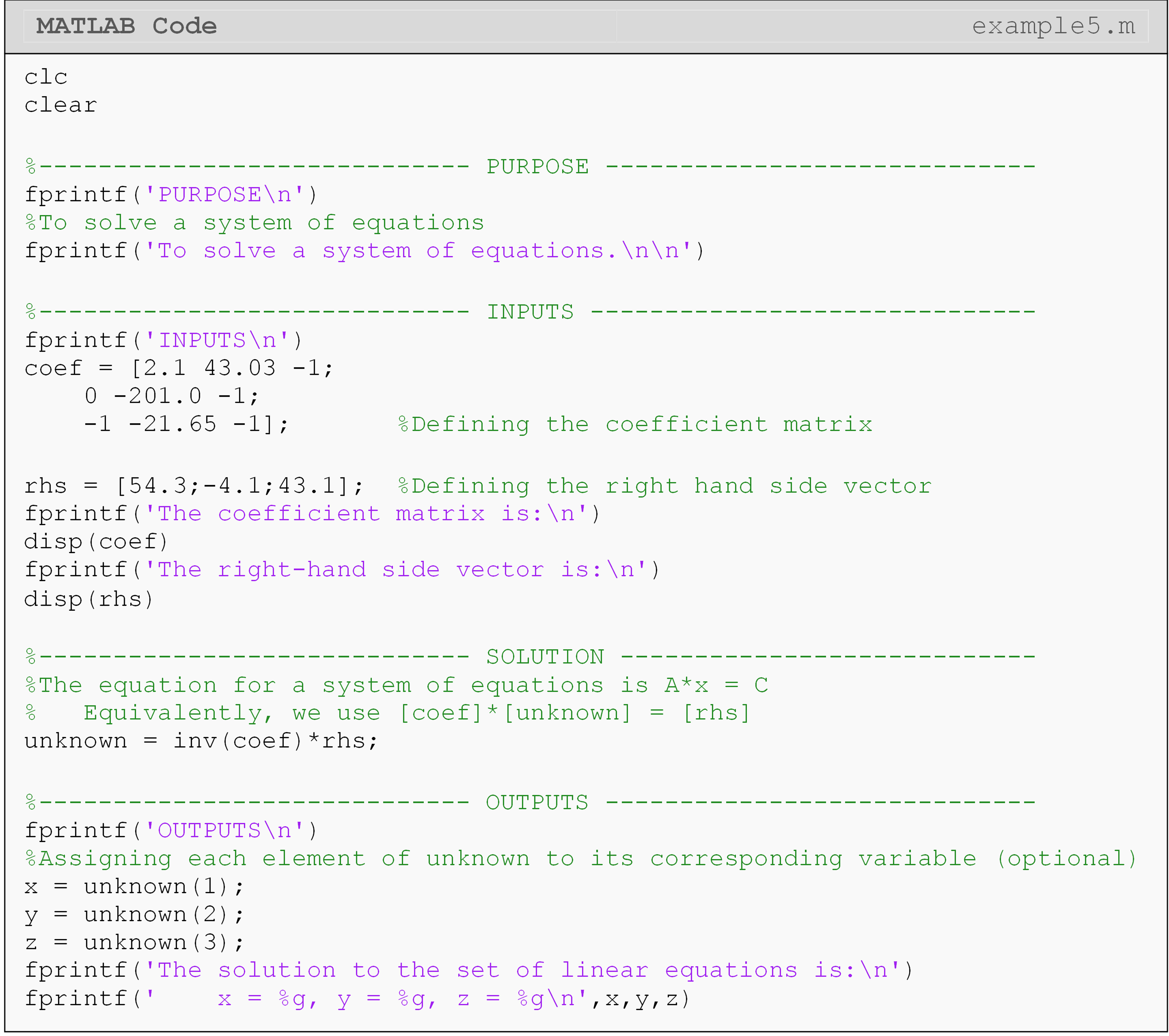
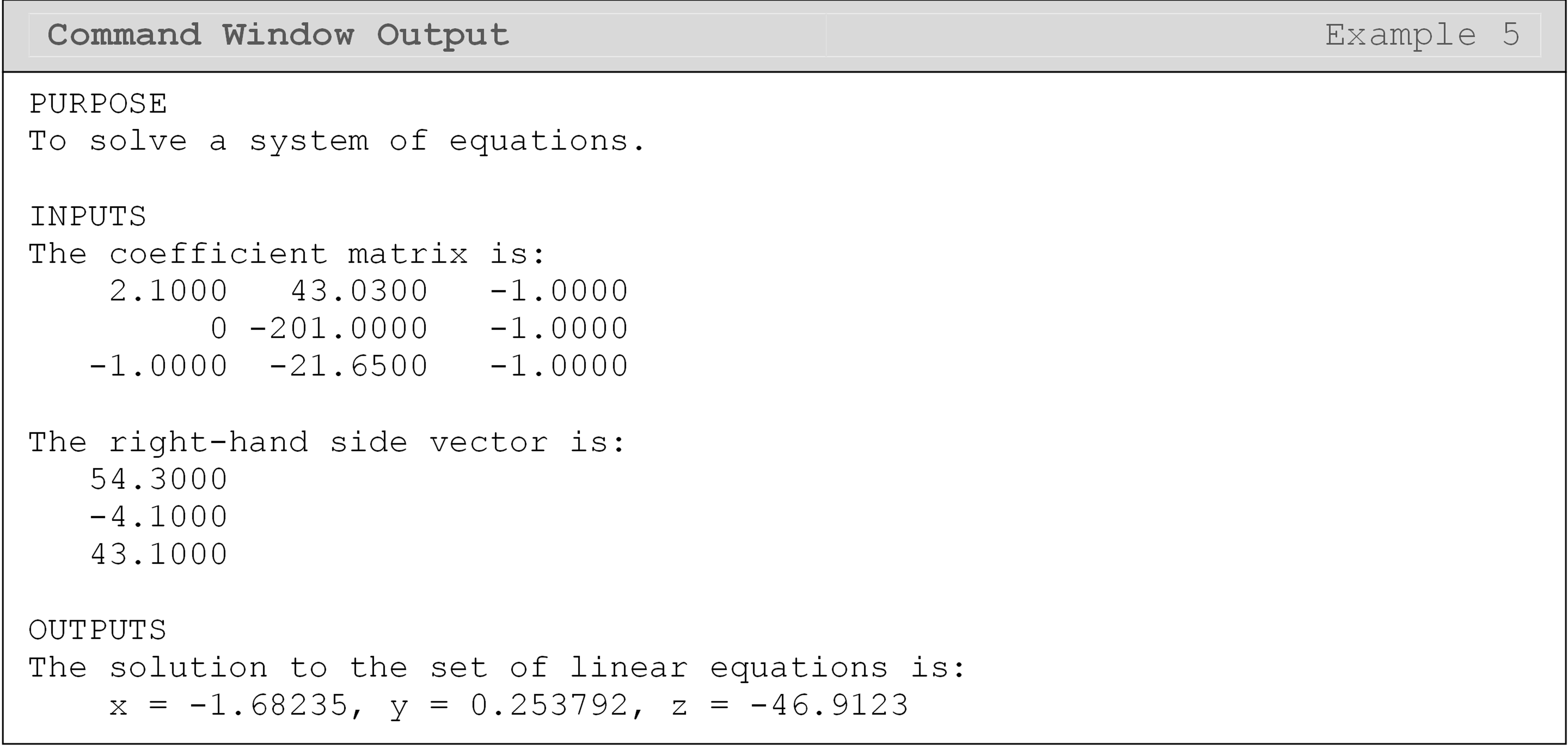
Example 5
A coworker is having trouble solving a system of 3 equations with 3 unknowns and has asked for your help. You tell them “I’ll have the system of equations solved for you before lunch!”
The equations are
\[{z = 2.1x + 43.03y - 54.3 }\\{z = - 201.0y + 4.1 }\\{z = - x - 21.65y - 43.1}\]
Solution
Rewrite the equations so that the unknown variables are on the left side and the known constants are on the right side:
\[{2.1x + 43.03y - z = 54.3 }\\{- 201.0y - z = - 4.1 }\\{- x - 21.65y - z = 43.1}\]
The set of equations can be written in matrix form as
\[\begin{bmatrix} 2.1 & 43.03 & -1\\ 0 & -201.0 & -1\\ -1 & -21.65 & -1\end{bmatrix} \begin{bmatrix} x \\ y\\ z\end{bmatrix} = \begin{bmatrix} -54.3\\ -4.1\\ 43.1\end{bmatrix}\]
This system of equations has been annotated for clarity in Figure 7. Each of the three arrays (coefficient matrix, solution vector, right-hand side vector) are labeled.
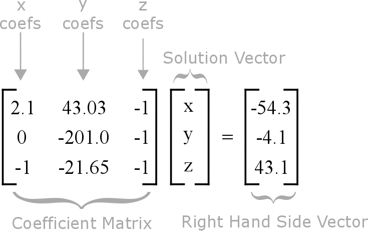
Figure 7: Annotated system of equations for Example 5.
Now that the coefficient matrix, the right-hand side, and solution
vectors are found, one can write a program to solve the system of
equations. Functions listed previously in this lesson, such as the
inverse function, inv(), are used to help solve this system of
equations.
As mentioned above, matrix division is not defined, which is why we used
the inv() function in Example 5. This is categorically true. However,
MATLAB has implemented a more efficient method for solving systems of
equations of the form \([A]\cdot[B]=[C]\), which does not use the inverse
of a matrix. This is of the form x = A\C or x = mldivide(A,C): these
two are equivalent syntax in MATLAB. Note that these are not
replacements for calculating the inverse of a matrix.
In Example 6, we solve a system of equations (of the form
\([x]\cdot[A]=[C]\)) using the x = A\C syntax. If you have a system of
equations of the form x*A = C, you should solve using x = A/C.
Remember, the order of matrix multiplication is not commutative, so
these two cases require different solutions.
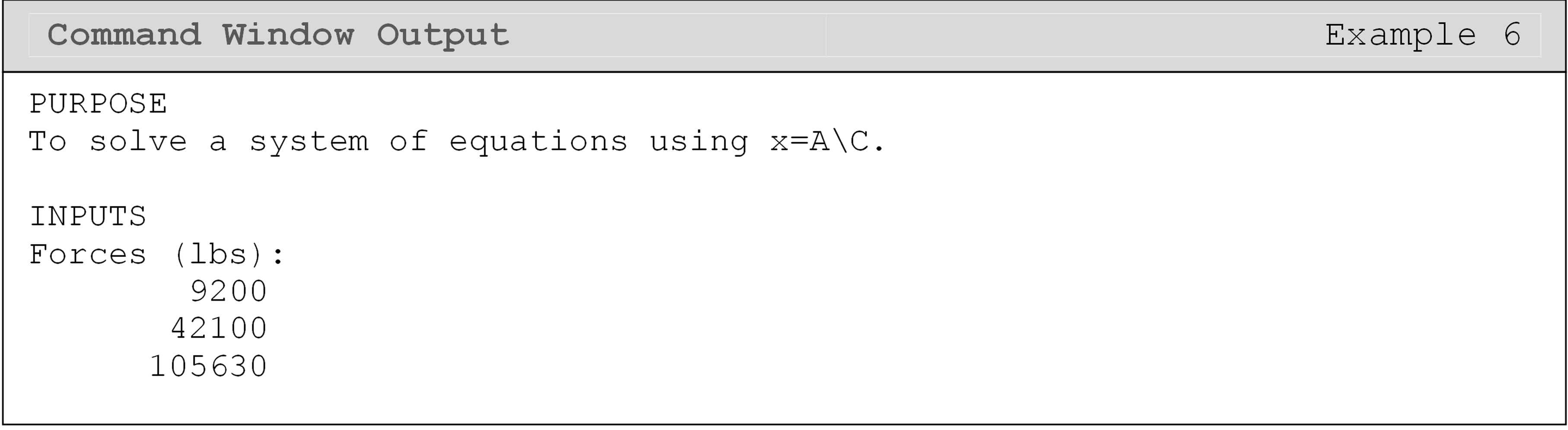
Example 6
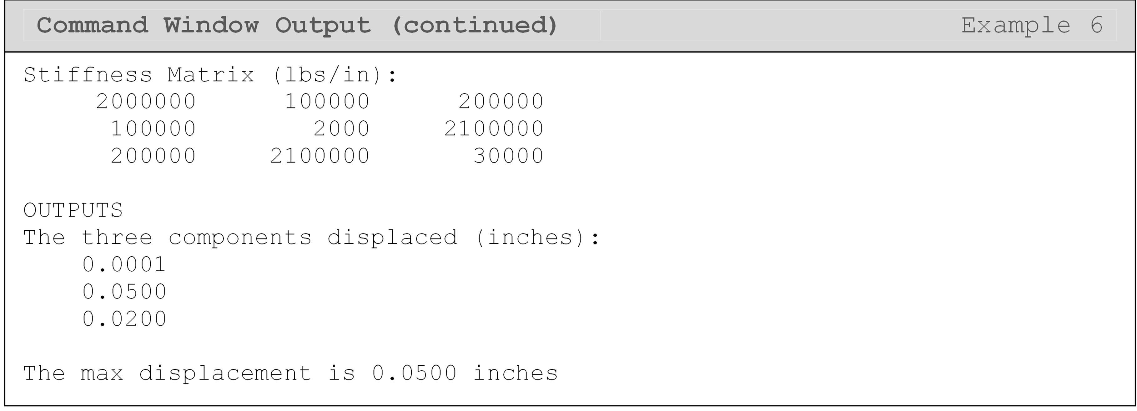
The amount of force that is exerted on a body can be determined by measuring the amount that the body displaces, and vice-versa. Ultimately, this force value can help determine the amount of stress acting on and inside the body or structure. This method for determining stress is widely used in finite element modeling and is also applicable to a variety of other systems (heat transfer, vibration analysis, etc.). Typically, the force and displacement values are modeled as vectors, and they are related to each other through the stiffness matrix. The relationship of the force, displacement, and stiffness matrices is
\[\lbrack\overset{\rightarrow}{F}\rbrack = \lbrack k\rbrack\ \lbrack\overset{\rightarrow}{x}\rbrack\]
where,
F is the force column vector.
k is the stiffness matrix.
x is the displacement column vector.
For each system, the stiffness matrix is different and is dependent on the material properties and the system component geometry in use. Given the stiffness matrix (\([k]\), lbs/in), find the displacement (inches) of all three components if each component has a normal force acting on it as listed (use relationship given above). The element forces are: 9200, 42100, 105630 lbs.
The stiffness matrix is
\[\left\lbrack k \right\rbrack = \begin{bmatrix} \text{2} & \text{0.1} & \text{0.2} \\ \text{0.1} & \text{0.002} & \text{2.1} \\ \text{0.2} & \text{2.1} & \text{0.03} \\ \end{bmatrix} \times \text{10}^{\text{3}}\ \text{kip/in}\]
Output the maximum value of the displacement vector elements with a brief description.
Solution
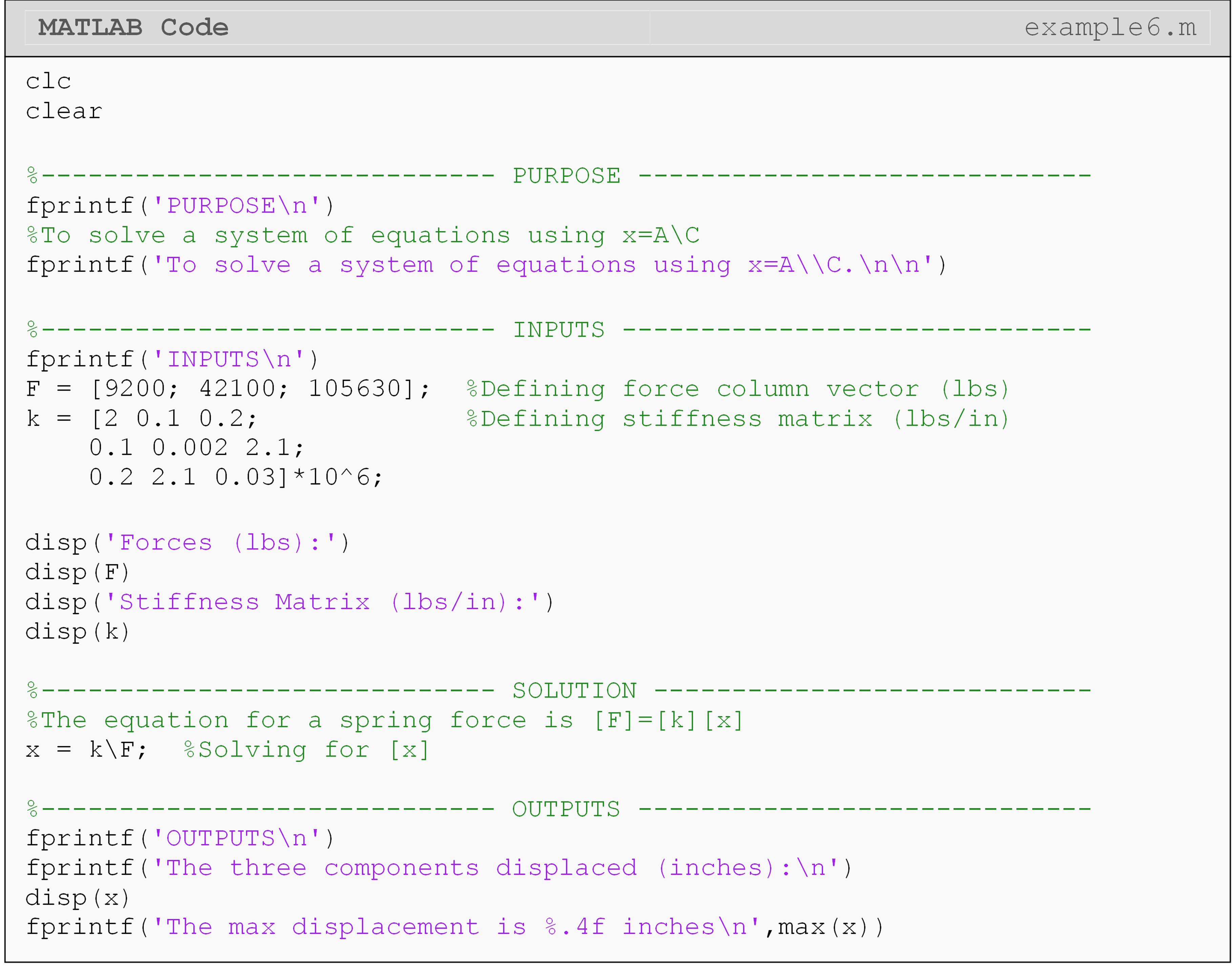
It is important to note that MATLAB does not account for units, so one must be very careful when solving engineering problems. This example shows a basic way to solve a problem that uses the finite element method (FEM). It should be noted that the element stiffness matrix for most finite element problems is of very large size, but the matrix operations are essentially the same as shown in Example 6.
Lesson Summary of New Syntax and Programming Tools
| Task | Syntax | Example Usage |
| Solve A*x = C for x | mldivide() or \ |
mldivide(A,C) or A\C |
| Solve x*A = C for x | mrdivide() or / |
mrdivide(C,A) or C/A |
| Matrix addition | + |
A+B |
| Matrix subtraction | - |
A-B |
| Matrix multiplication | * |
A*B |
| Array operations | . |
A.*B |
| Matrix inverse | inv() |
inv(A) |
| Raise a matrix to a power | ^ |
A^2 |
| Vector dot product | dot() |
dot(A,B) |
| Vector cross product | cross() |
cross(A,B) |
| Matrix transpose | ' or transpose() |
A' |
| Find the smallest element | min() |
min(A) |
| Find the largest element | max() |
max(A) |
| Sort an array | sort() |
sort(A) |
| Matrix determinant | det() |
det(A) |
| Norm of a matrix | norm() |
norm(A,type) |
| Trace of a matrix | trace() |
trace(A) |
Multiple Choice Quiz
(1). The array operator (.) in MATLAB is used for
(a) conducting element-by-element matrix operations
(b) conducting matrix multiplication
(c) denoting a decimal point
(d) finding the dot product of vectors
(2). The function to find the determinant of a matrix \([A]\) is
(a) |A|
(b) det(A)
(c) determinant(A)
(d) determ(A)
(3). When subtracting two matrices, the matrices must have
(a) equal inner dimensions
(b) zeros along the diagonal
(c) unequal sizes
(d) equal sizes
(4). Which of the following will give the transpose of a matrix \([A]\) in MATLAB?
(a) trans(A)
(b) transpose(A)
(c) A'
(d) Both b & c
(5). When multiplying two matrices, the matrices must have
(a) equal sizes
(b) zeros along the diagonal
(c) unequal sizes
(d) equal inner dimensions
Problem Set
(1). Given
\[[A] = \begin{bmatrix} 5 & 2 & 4 \\ -2 & 3 & 1 \\ 7 & 2 & -1 \end{bmatrix} \ \ [B] = \begin{bmatrix} 4 & -3 \\ 6 & 2 \\ -4 & 1 \end{bmatrix} \ \ [C] = \begin{bmatrix} 6 & 9 \\ 5 & -2 \\ 1 & 4 \end{bmatrix}\]
use MATLAB to find
(a) \([B] + [C]\)
(b) \([B] - [C]\)
(c) inverse of \([A]\)
(d) \([A][B]\)
(e) \(\displaystyle\text{det}(A)\)
(f) \(\displaystyle[A]^T\)
(g) The square of each element of \([A]\)
(h) The natural log of each element of \([A]\)
(2). Using matrices and MATLAB, solve for the variables x,y,z in the system of linear equations.
\[3x + 5y - 2z = 1 \\2x - 2y + 7z = 3 \\x + 8y - 4z = - 6\]
Use fprintf() to display the solution to the system of equations.
Include a brief description of the solution as well.
(3). Given that the equation of a line is \(y = mx + b\) where m is the slope and b is the vertical (y-intercept), use matrices to find the equation of the line that passes through the (x,y) data pairs: (1,6) and (4,10).
(4). Given
\[\lbrack P\rbrack = \begin{bmatrix} 4 & 0 & - 3 & 7 \\ 9 & 7 & 4 & 2 \\ 0 & 1 & - 9 & 6 \\ 3 & 2 & 7 & 1 \\ \end{bmatrix}\]
use MATLAB to find the
(a) row and column dimensions using the size() function.
(b) infinity norm of \([P]\)
(c) trace of \([P]\).
(d) inverse of \([P]\), and name the matrix, Q.
For parts (a), (b) and (c), use fprintf() to display the result.
For (d), use disp() to display Q.
(5). Given the two vectors,
\[{\overset{\rightarrow}{\omega} = \begin{bmatrix} 4 & 2 & 7 \\ \end{bmatrix}} \\ {\overset{\rightarrow}{r} = \begin{bmatrix} 2.5 & 4 & 1.3 \\ \end{bmatrix}}\]
use MATLAB to find the
(a) vector dot product.
(b) vector cross product.
(c) sorted vector of \(\overset{\rightarrow}{r}\), and name the array, rSort.
Use the fprintf() or disp() functions to display the appropriate
solution(s).