Module 4: MATH AND DATA ANALYSIS
Learning Objectives
After reading this lesson, you should be able to:
(1) perform basic algebra with mathematical operators,
(2) find logarithmic functions with different bases in MATLAB,
(3) calculate basic trigonometric functions in MATLAB.
What kind of mathematical functions and operations are available in MATLAB?
Basic math (addition, subtraction, multiplication, etc.) syntax in
MATLAB is the same as it is in most calculators (+,-,*,/,^). The
syntax is the same whether used with variables or directly with numbers.
You have seen these numerous times in previous lessons, but we include
them here for completeness.
 Important Note: You must
use the multiplication operator everywhere you have multiplication.
\(7x\) should be
Important Note: You must
use the multiplication operator everywhere you have multiplication.
\(7x\) should be 7*x, and \(7(x+1)\) should be 7*(x+1). You will get
an error if you are missing a multiplication operator.
MATLAB has several mathematical functions such as logarithmic, exponential, trigonometric, hyperbolic, etc. In this lesson, we will cover the use of logarithmic and trigonometric functions.
How do I use logarithmic functions in MATLAB?
The first function that is presented is the log() function. This
function is only for the natural logarithm.
The inverse of a natural log function is the exponential function. You
cannot use log^-1 in MATLAB to find the inverse of a natural
log. The function to find the value of an exponential function is
exp().
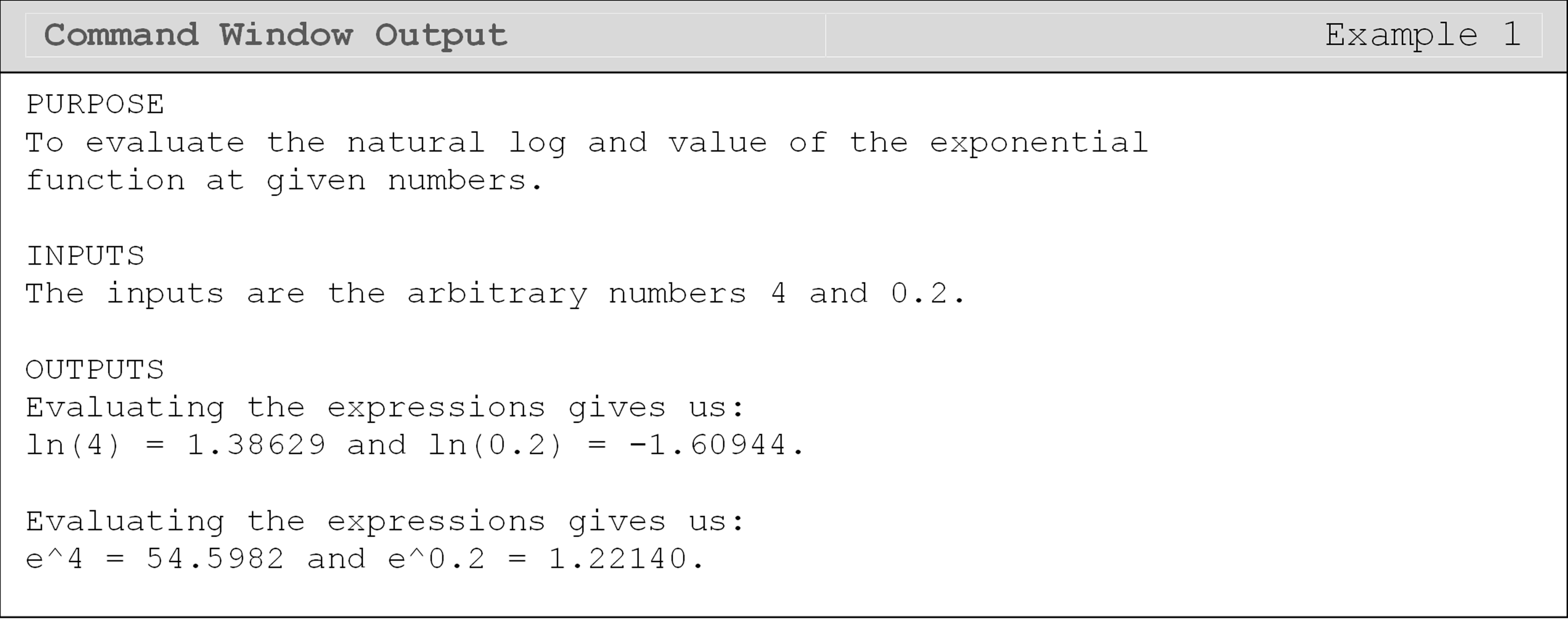
Example 1
Find the natural log of 4 and 0.2, and name these outputs \(y1\) and \(y2\), respectively. Find the value of the exponential function of both \(y1\) and \(y2\), and examine the results.
Solution
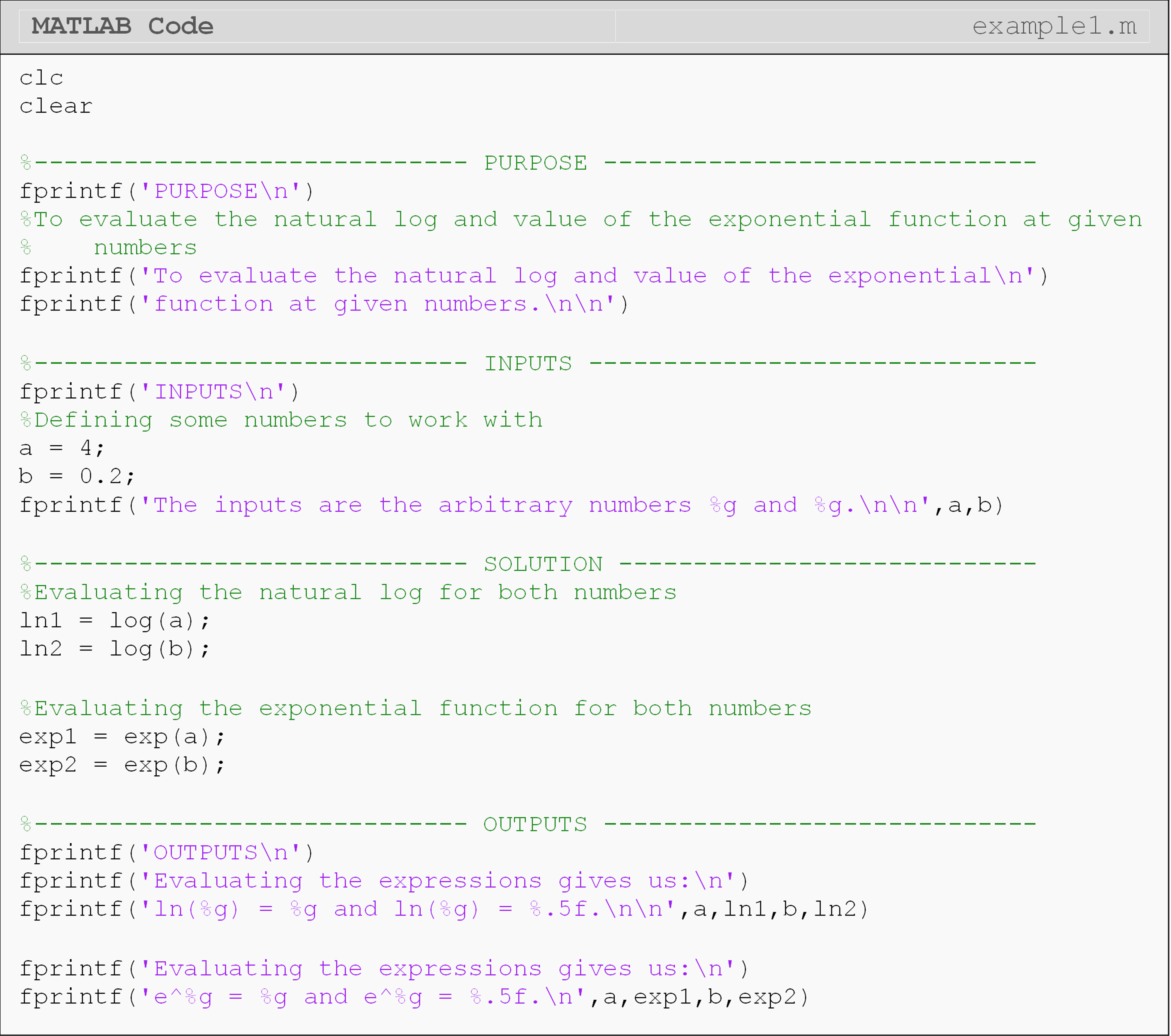
Note that when typing the function exp(num), it cannot be substituted by exp^num, as this will give you a syntax error as given below.
??? Error using ==> exp
Not enough input arguments.
What about a logarithm that is not natural?
Besides the natural logarithm, one of the most common logarithms is log
with the base 10. The function to find a log with a base of 10 is
log10().
To find the value of a logarithm that does not have a base of 10 or e (natural log), you may use the change of base formula. To simplify the m-file when using the change of base formula, it is recommended that you use natural logs to change the base. The formula for the log of b with the base a is,
\[ \text{log}_{a}(b)=\frac{\text{ln}(b)}{\text{ln}(a)} \]
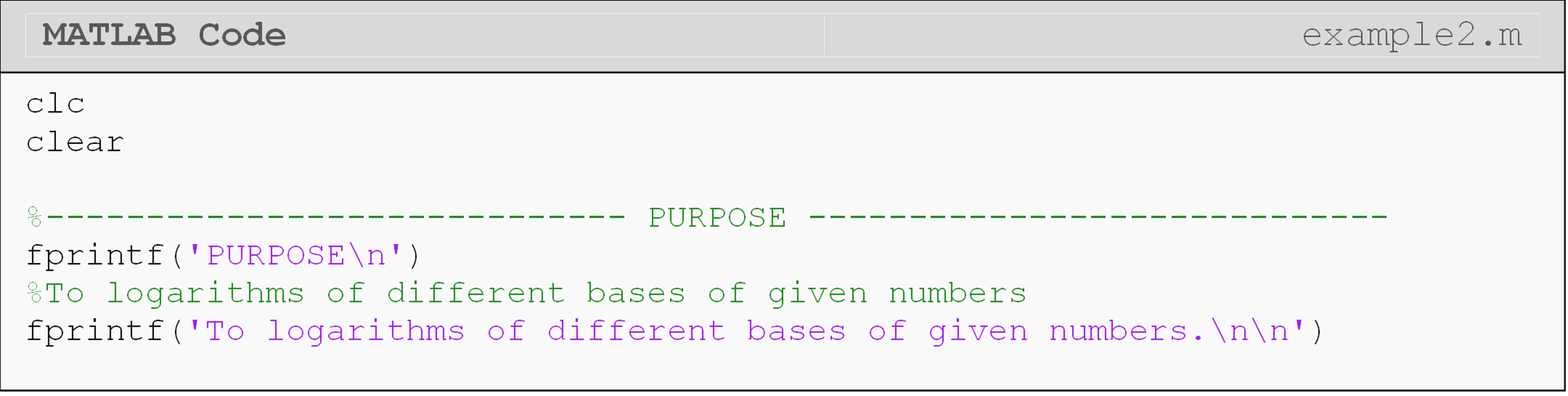
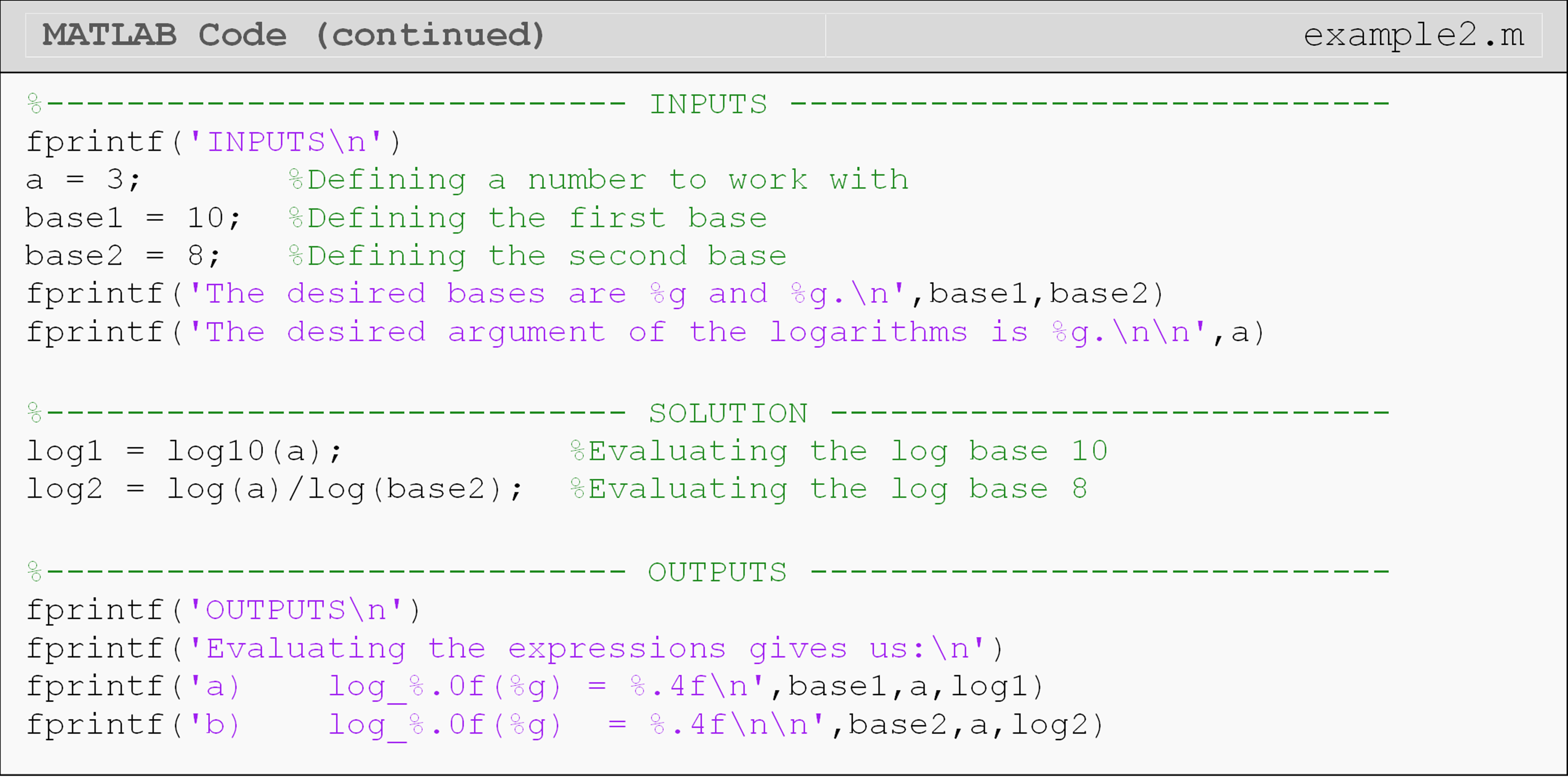
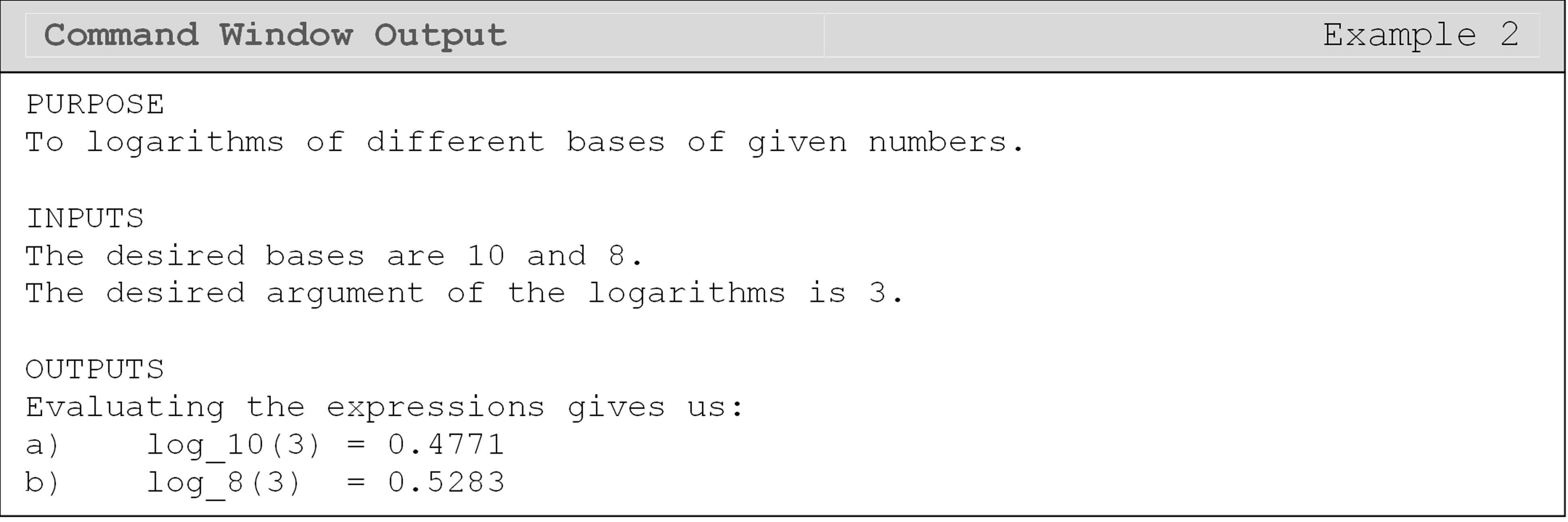
Example 2
Using MATLAB, find:
(a) \(\text{log}_{10}(3)\)
(b) \(\text{log}_{8}(3)\)
Use the fprintf() function to describe the outputs in the Command Window. Hint: Consider using the change of base formula for part (b).
Solution
Note the different code used for finding the natural log (Example 1) and the log with a different specified base (Example 2). The functions for natural log, exponential function, and log10 can all be found in Table 1 at the end of this lesson.
How can MATLAB evaluate trigonometric functions?
MATLAB has several trigonometric functions. However, note that the input for these trigonometric functions is in radians: not degrees.
The function to find the cosine of an angle is cos(). This function
assumes an input of an angle in radians. The functions for sine,
tangent, cosecant, secant, and cotangent are sin(), tan(), csc(),
sec(), and cot(), respectively. These functions have the same inputs
and usage as the cos() function shown above (see Table 1).
If you wish to input the argument to a trigonometric function in
degrees, attach a d to the end of the function. For example, to find the
value of the cosine of 30 degrees, you may type, cosd(30).
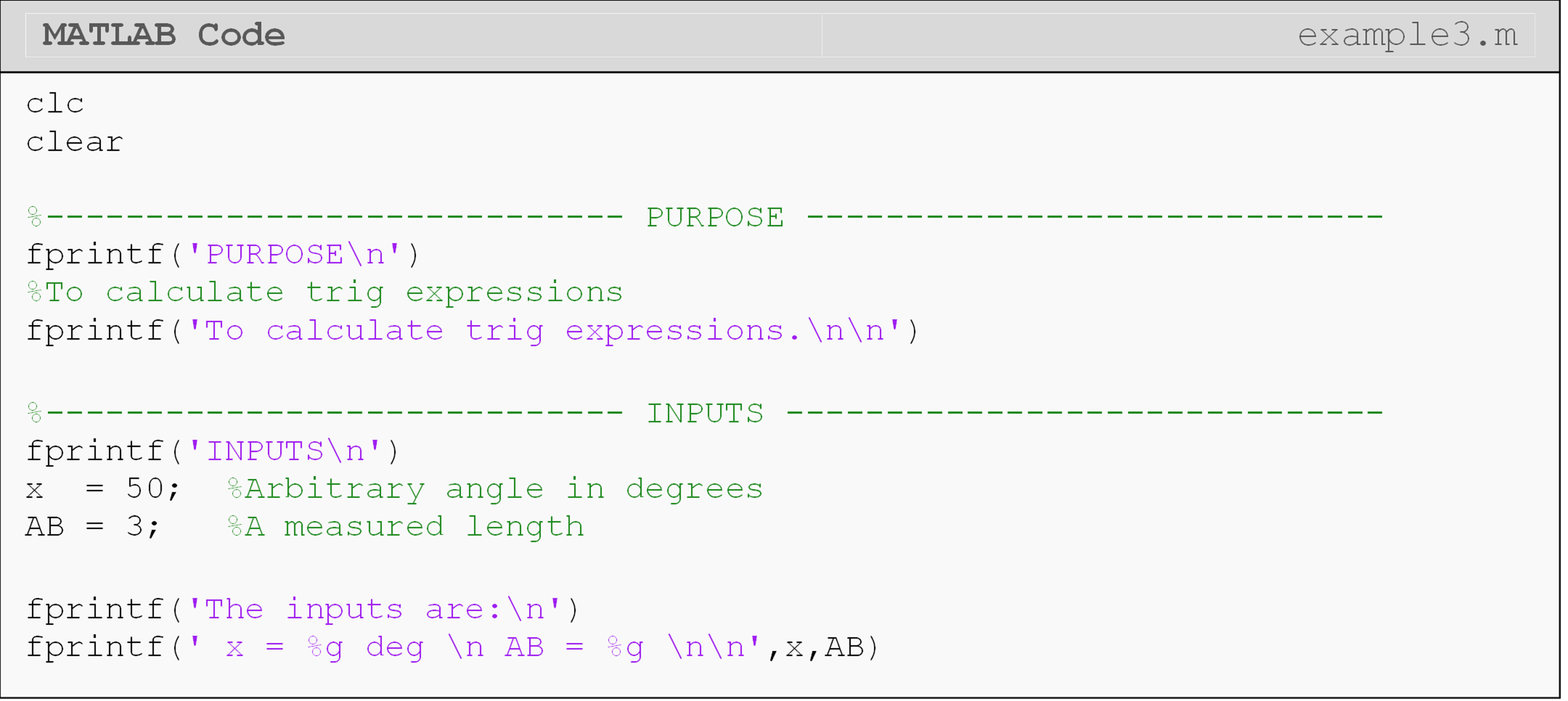
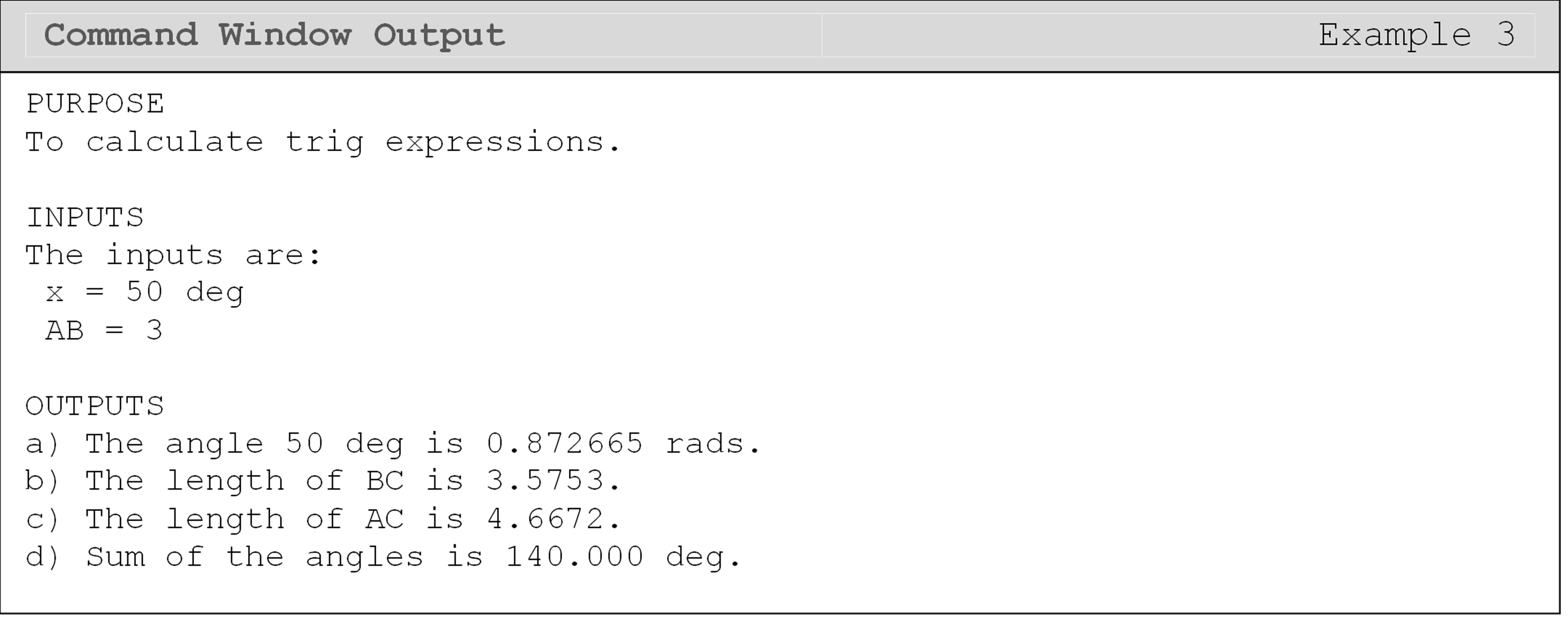
Example 3
A right-angled triangle ABC, shown in Figure 3, with \(x = 50^{\circ}\) and \(\overline{\text{AB}}\) = 3 is given.
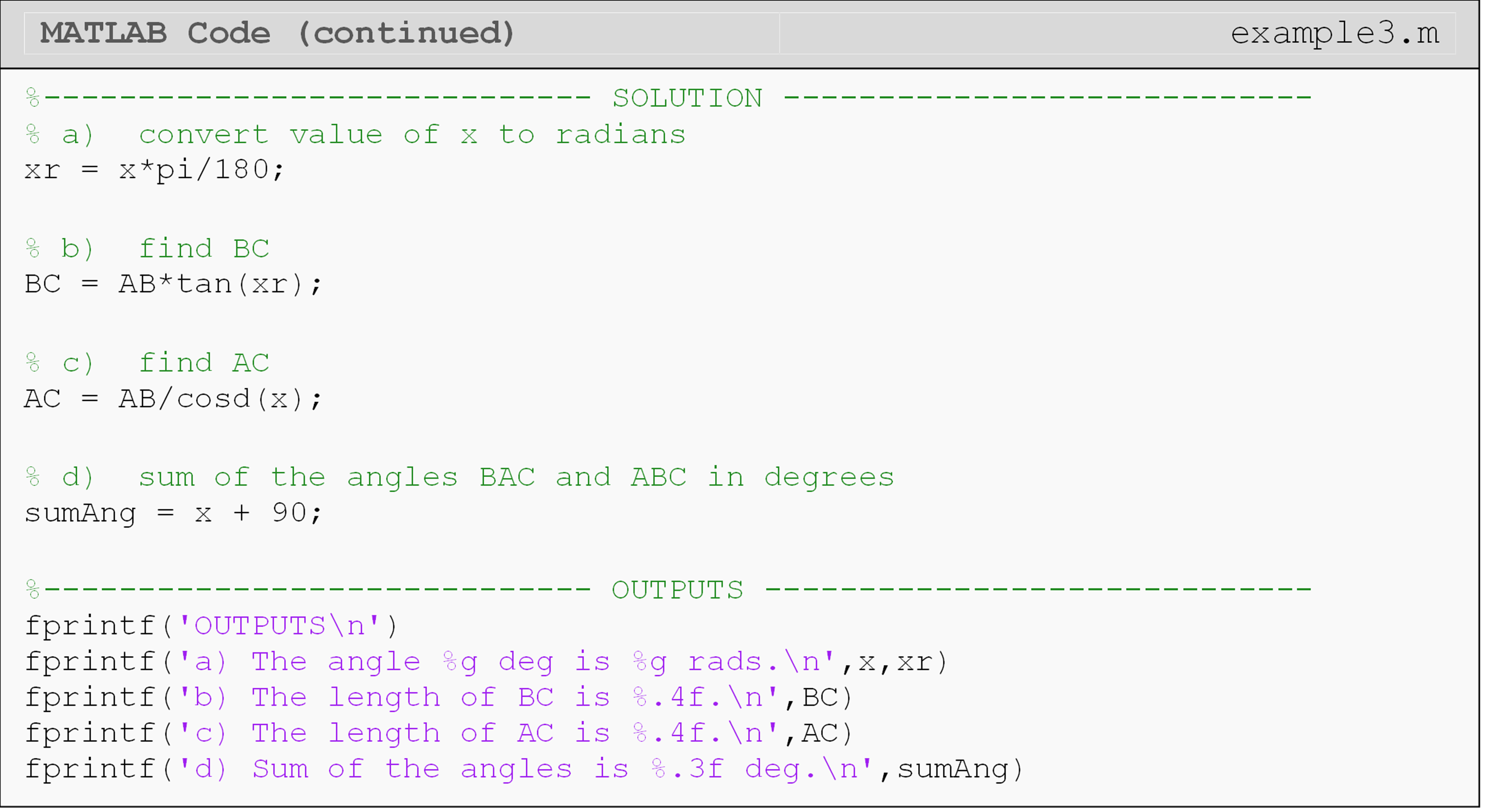
(a) Convert x to radians.
(b) Find \(\overline{\text{BC}}\).
(c) Find \(\overline{\text{AC}}\).
(d) What is the sum of \(\angle\)BAC and \(\angle\)ABC in degrees?
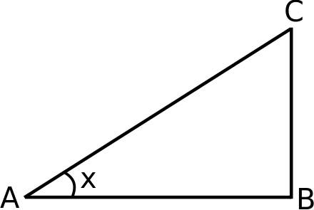
Figure 1: The Command Window output for Example 3.
All outputs should be displayed in the Command Window using the
fprintf() or disp() functions.
Solution
Notice, in the example code, that MATLAB stores the numeric value of
\(\pi\) in the predefined variable pi. Also take a look at the method to
convert the value of x from degrees to radians for part a (if you are
not familiar with it). Be sure that the argument for all applicable
trigonometric functions is in radians or add a d for degrees (e.g.,
sind(30)) as mentioned previously.
Lesson Summary of New Syntax and Programming Tools
| Task | Syntax | Example Usage |
|---|---|---|
| Find the natural log of a number | log() |
log(a) |
| Evaluate the exponential function at a number | exp() |
exp(a) |
| Log with base 10 | log10() |
log10(a) |
| Sine of an angle | sin() |
sin(a) |
| Cosine of an angle | cos() |
cos(a) |
| Tangent of an angle | tan() |
tan(a) |
| Cosecant of an angle | csc() |
csc(a) |
| Secant of an angle | sec() |
sec(a) |
| Cotangent of an angle | cot() |
cot(a) |
| Sine inverse of a number | asin() |
asin(a) |
| Cosine inverse of a number | acos() |
acos(a) |
| Tangent inverse of a number | atan() |
atan(a) |
| 4 quadrant tan inverse complex number | atan2() |
atan2(Im,Re) |
Multiple Choice Quiz
(1). The function for finding the natural log of a number is
(a) ln()
(b) log()
(c) loge()
(d) nlog()
(2). The function for finding the exponential function of a number is
(a) e()
(b) e\^()
(c) exp()
(d) exp\^()
(3). The function to find the value of sin(a) where a is \(34^\circ\), is
(a) sin(34)
(b) sine(34)
(c) sin((34\*180)/pi)
(d) sin((34\*pi)/180)
(4). The function acos()
(a) determines if the cosine value can be evaluated.
(b) evaluates the cosine of an angle in degrees.
(c) evaluates the cosine of an angle in radians.
(d) evaluates the inverse cosine of an argument.
(5). The sind() function
(a) determines if the sine value can be evaluated.
(b) evaluates the inverse sine of an argument.
(c) evaluates the sine of an angle given in degrees.
(d) evaluates the sine of an angle given in radians.
Problem Set
(1). Given that \(a=7\), \(b=2\), and \(c=11\), using MATLAB, find the values of
(a) \(\text{log}_{10}(b)\)
(b) \(b\text{ln}(c)\)
(c) \(e^{-\frac{a}{2}}\)
(d) \(\text{log}_2(a)\)
Output each solution to the Command Window, and check your results using a calculator.
(2). The approximate value of \(e^x\) (exponential function) can be found by using a finite number of terms of the following infinite Maclaurin series,
\[e^x = 1+x+\frac{x^2}{2!}+\frac{x^3}{3!}+\text{...} \]
for all \(x\).
Complete the following using \(x=2.3\):
(a) Compare the output of the first 3 terms for the Maclaurin series for exponential function against the MATLAB output for the exponential function.
(b) Redo part (a) using first 6 terms of the Maclaurin series.
Make sure to use the fprintf() or disp() functions to display your
program outputs in the Command Window.
(3). Given the triangle ABC, shown in Figure A, with angles \(\theta_1 = \frac{\pi}{8}\text{ radians,}\ \theta_{2} = \text{34}^\circ\text{, and length }\overline{\text{AB}} = 11\), find the following.
(a) \(\theta_3\) in degrees
(b) \(\overline{\text{BC}}\)
(c) \(\overline{\text{AC}}\)
(d) area of triangle ABC
Hint: The law of cosines is given as
\[\frac{\overline{\text{AB}}}{\sin(\theta_1)} = \frac{\overline{\text{BC}}}{\sin(\theta_2)} = \frac{\overline{\text{AC}}}{\sin(\theta_3)}\]
The area of a triangle is
\[A = \sqrt{s(s-a)(s-b)(s-c)}\]
where s = semi-perimeter of the triangle and a, b, c = length of the three sides of the triangle
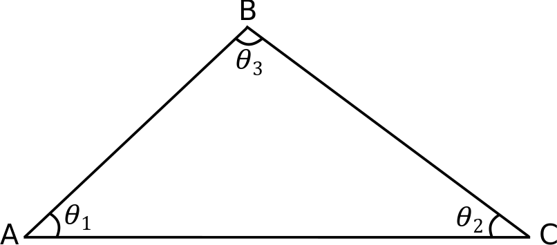
Figure A: Labeled triangle ABC is shown (not to scale).
Output each solution to the Command Window and verify your results >
with a calculator. Make sure to use the fprintf() or disp()
functions > to display your program outputs in the Command Window.
(4). The approximate value of \(\text{sin}(x)\) can be calculated using a finite number of terms of the following infinite Maclaurin series
\[ \text{sin}(x) \approx x - \frac{x^3}{3!} + \frac{x^5}{5!} - \frac{x^7}{7!} \] for all x. Complete the following using \(38^\circ\)
(a) Compare the output of the first 3 terms of the Maclaurin series
provided, against the MATLAB output for the sine command.
(b) Redo part (a) using the first 5 terms of the series.
Make sure to use the fprintf() or disp()` functions to display your
program outputs in the Command Window.
(5). The mechanical components of a certain suspension system dynamically respond to an applied force by vibration. The actual position, x(t), of the center of mass of the system as a function of time, t, is given by,
\[ x(t)=Xe^{\xi{}\omega{}_{\text{n}}t}(\text{cos}(\sqrt{1-\xi{}^2}\omega{}_{\text{n}}t)) \]
Ideally, the center of mass would follow the following position function,
\[ x(t)=Xe^{-\xi\omega{}_{\text{n}}t} \]
Given that \(X=2,\) \(f_{\text{n}}=1.3\) \(\omega_{\text{n}}=2\pi{}f_{\text{n}}\) \(\xi=0.1\)
Plot the actual and the ideal position of the system as a function of time. Use a legend, give axis and graph titles, and use reasonable line thicknesses and symbols. Plot the position for the time from 0 to 8 seconds in a single plot where the horizontal axis is the time and the vertical axis is the position of the center of mass.