Module 4: MATH AND DATA ANALYSIS

Lesson 4.9 – Ordinary Differential Equations

Learning Objectives

After reading this lesson, you should be able to:

solve an ordinary differential equation using MATLAB.

What is a differential equation?

An equation that consists of derivatives is called a differential equation. Differential equations have applications in all areas of science and engineering. A mathematical formulation of most physical and engineering problems leads to differential equations. So, it is important for engineers and scientists to know how to set up differential equations and solve them. Differential equations are of two types:

ordinary differential equations (ODE) and
partial differential equations (PDE).

An ordinary differential equation is that in which all the derivatives are with respect to a single independent variable. Examples of ordinary differential equations include:

\(\displaystyle\frac{d^2y}{dx^2} + 2\frac{dy}{dx} + y = 0\), \(\displaystyle\frac{dy}{dx}(0) = 2,\ \ y(0) = 4\),
\(\displaystyle\frac{d^3y}{dx^3} + 3\frac{d^2y}{dx^2} + 5\frac{dy}{dx} + y = \sin x,\) \(\displaystyle\frac{d^2y}{dx^2}(0)=12\) \(\displaystyle\frac{dy}{dx}(0)=2\), \(y(0) = 4\)
\(\displaystyle\frac{d^2y}{dx^2}-5y=6(100-x)\), \(\displaystyle y(0)=5\), \(\displaystyle y(100)=27\)

Ordinary differential equations are classified in terms of order and degree. The order of an ordinary differential equation is the same as the highest derivative and the degree of an ordinary differential equation is the power of the highest derivative. Thus, the differential equation,

\[\displaystyle x^3\frac{d^3y}{dx^3}+x^2\frac{d^2y}{dx^2}+x\frac{dy}{dx}+xy=e^x\]

is of order 3 and degree 1, whereas the differential equation

\[\displaystyle \left( \frac{dy}{dx}+1 \right)^2+x^2\frac{dy}{dx}=\sin x\]

is of order 1 and degree 2.

How do I set up and solve a differential equation?

An engineer’s approach to differential equations is different from that of a mathematician. While the latter is interested in the mathematical solution, an engineer should be able to interpret and implement the result physically. So, an engineer’s approach can be divided into three phases:

formulation of a differential equation from a given physical situation,
solving the differential equation using given conditions, and
interpreting the results physically for implementation.

To solve a differential equation, we need

the differential equation, deq,
the initial/boundary condition(s), IV, and
the independent variable, x.

In MATLAB, the function to solve an ordinary differential equation exactly is dsolve(). A usage example is dsolve(deq,IV,x). The number of initial or boundary conditions needed is the same as the order of the differential equation.

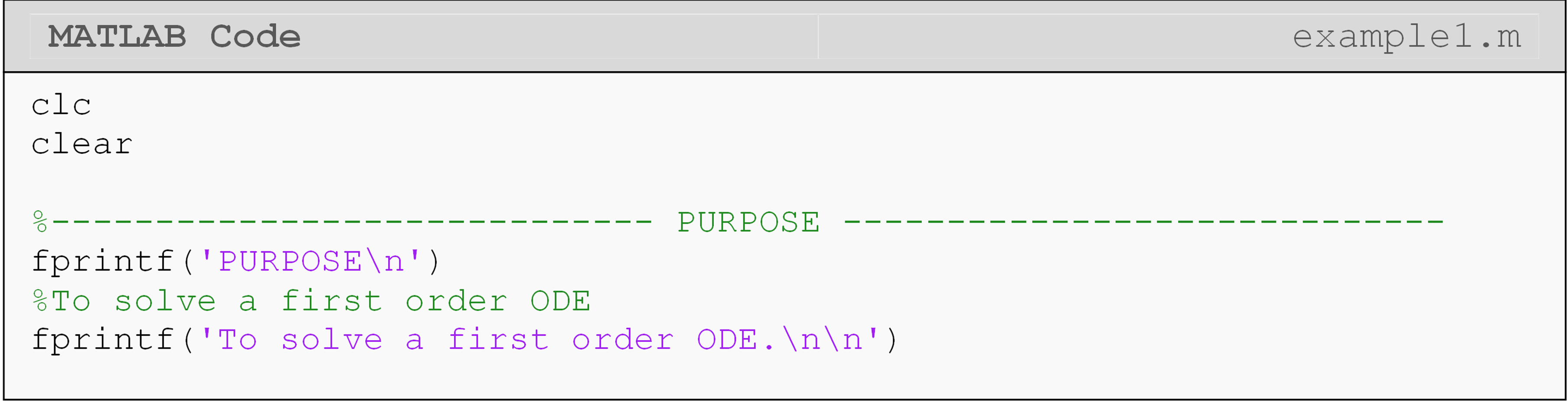
Example 1

Analytically solve the following differential equation using MATLAB.

\[\displaystyle2\frac{dy}{dx}=-3y+5e^x, \ \ y(0)=5\]

Solution

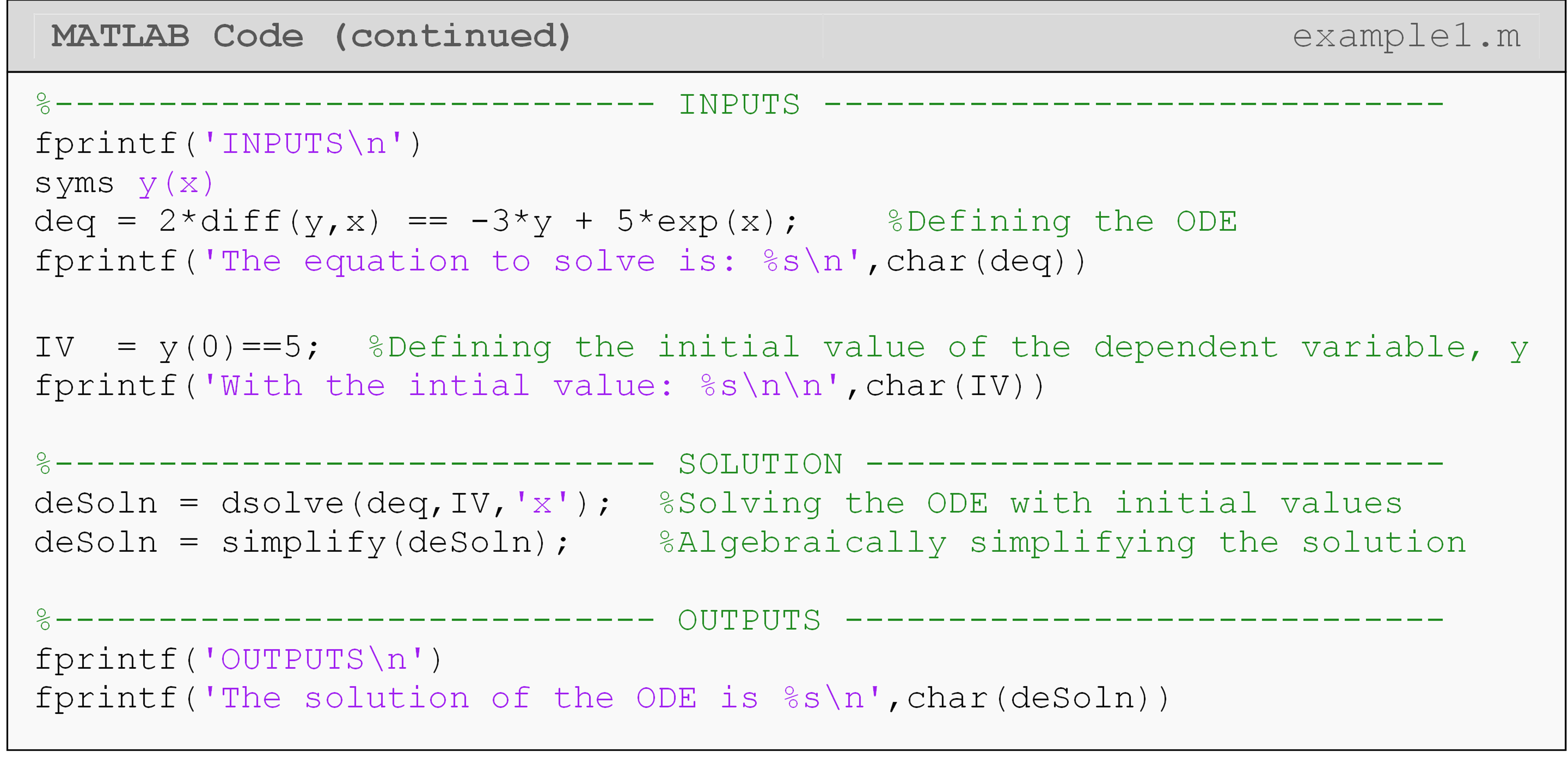
Note in Example 1 that the \(\displaystyle\frac{dy}{dx}\) part of the equation is entered as diff(y,x). This is possible because we have defined the symbolic function y(x). Therefore, both y and x are defined as symbolic variables in MATLAB. Also, note the use of the double equals (==) to separate the left- and right-hand sides of the differential equation. Recall that we used this same syntax when entering a left- and right-hand side of an equation when solving for its roots in Lesson 4.3. This must be done as MATLAB always associates a single equals sign (=) with assigning a value to a variable, which we have already done at the beginning of that line (deq =). In other words, when entering an equation with a left- and right-hand side, use double equals.

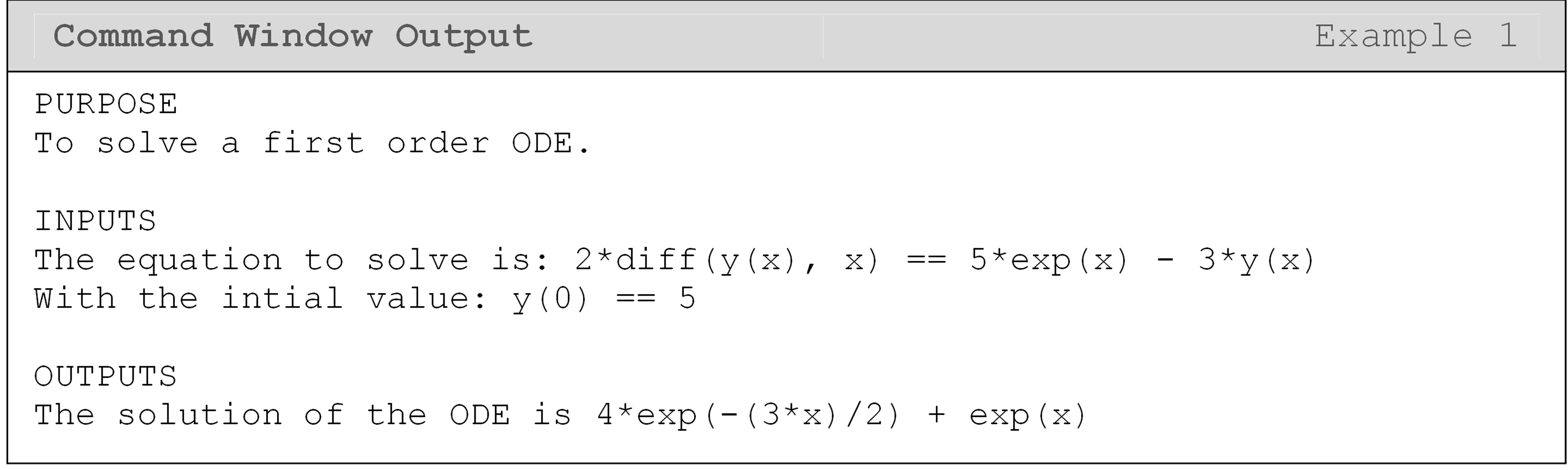
The simplify() function, in Example 1, is used to make the output aesthetically pleasing. It will try to algebraically simplify a mathematical expression that you give it as an input. Look at the code without simplify() to see the difference!

How do I solve a higher order ODE?

The dsolve() function is used to solve ordinary differential equations of all orders. However, you must make sure to place all the initial and boundary conditions correctly into the function. Look at Example 2 that shows how to solve a typical second order ordinary differential equation.

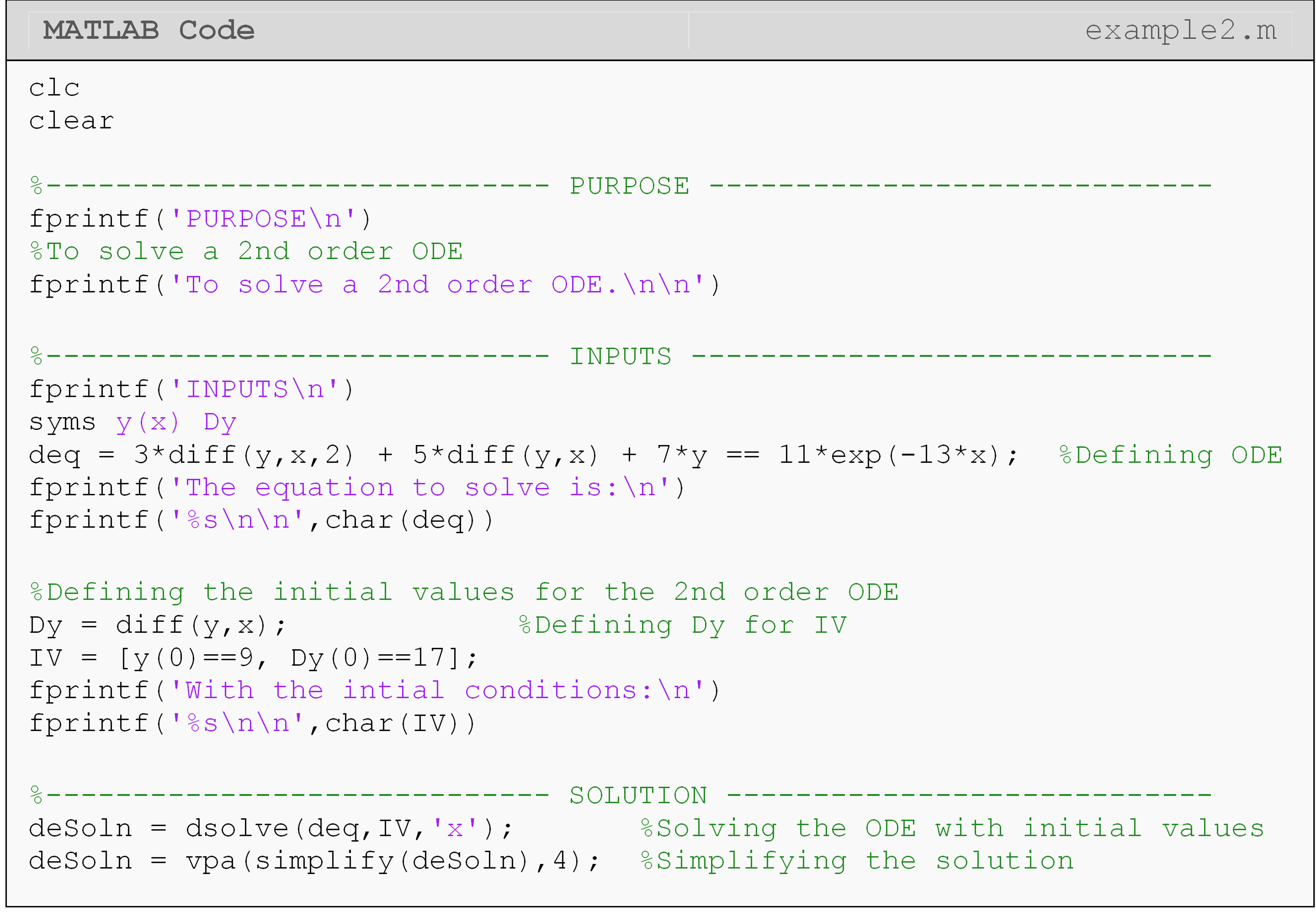
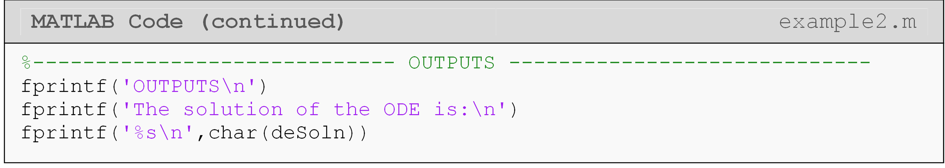
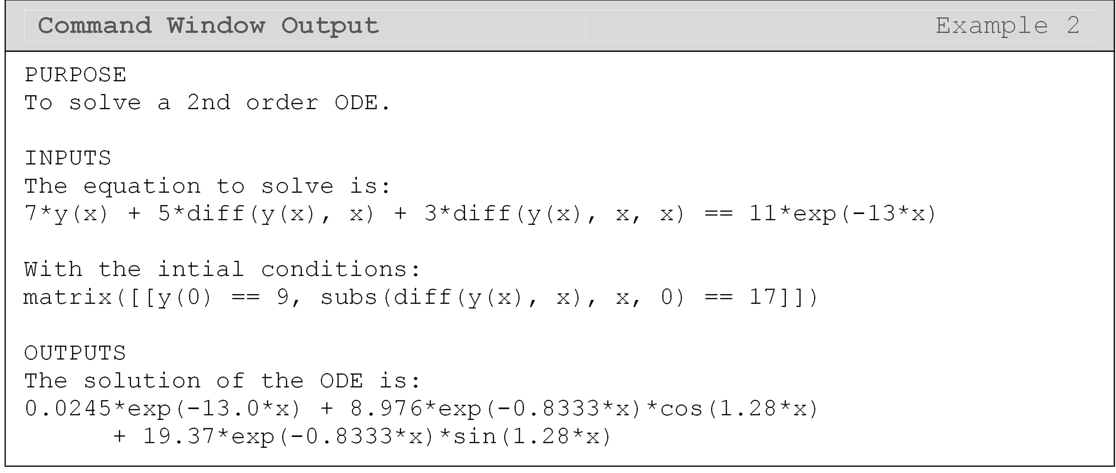
Example 2

Using the dsolve() function, solve the following ordinary differential equation.

\[\displaystyle3\frac{d^y}{dx^2}+5\frac{dy}{dx}+7y=11e^{-13x}, \ \ y(0)=19, \ \ \frac{dy}{dx}=17\]

Solution

When inputting the equation, look at how the \(\displaystyle\frac{d^2y}{dx^2}\) part of the equation is entered as diff(y,x,2). Other than that, the only changes made to the dsolve() function when compared to Example 1 are the number of initial values used to solve the differential equation. Since this ODE is second order, we require two initial values.

The solution to this differential equation is rather long, and one can see that using MATLAB to solve it saved some time and effort.

What are the limitations of using the `dsolve()` function?

As a programmer, one of the main pitfalls that you may experience is that the dsolve() function may not output a solution to a given differential equation. The dsolve() function uses symbolic manipulations to solve differential equations, and although very advanced, the algorithm cannot solve all ordinary differential equations (most do not have explicit solutions). You may receive this warning message in the Command Window:

Warning: Unable to find explicit solution.

If this is the case, solve the differential equation using a numerical method. Two (of the many) MATLAB functions that numerically solve a differential equation are ode45() and ode23(). For more information on using these functions, use the MATLAB documentation.

Lesson Summary of New Syntax and Programming Tools

Task	Syntax	Example Usage
Solve a differential equation analytically	`dsolve()`	`dsolve(deq,IV,x)`
Numerically solve a differential equation	`ode45()`	`ode45(deq,tspan,IV)`
Numerically solve a differential equation	`ode23()`	`ode23(deq,tspan,IV)`

Multiple Choice Quiz

(1). The MATLAB function for solving an initial value ordinary differential equation is

(a) ode()

(b) diff()

(d) diffsolve()

(2). The most appropriate choice for defining the following differential equation

\[7\frac{dy}{dt} + 3y = 4, \ \ y(0) = 2\]

for use with the dsolve() function is

(a) deq = 7diff(y,x) + 3*y == 4

(b) deq = 7Dy + 3y == 4

(d) deq = 7diff(y,x) + 3*y = 4

(3). Complete the code to solve the initial value ordinary differential equation.

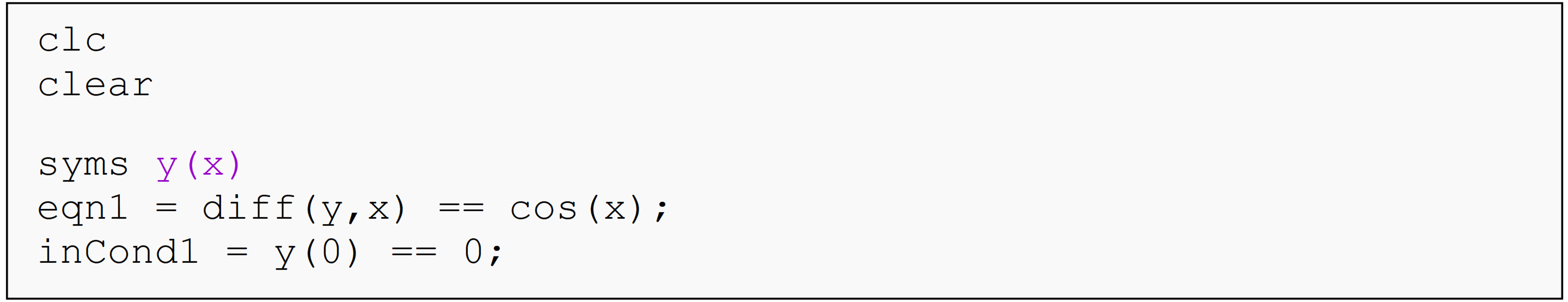
(a) dsolve(eqn1,inCond1,'x')

(b) dsolve(eqn1,inCond1,x)

(d) dsolve(inCond1,eqn1,'x')

(4). To solve

\[\displaystyle\frac{d^2y}{dx^2}=5x(30-x), \ \ y(0)=5, \ \ \frac{dy}{dx}(30)=7\] the most appropriate MATLAB line of code to add to the following program is

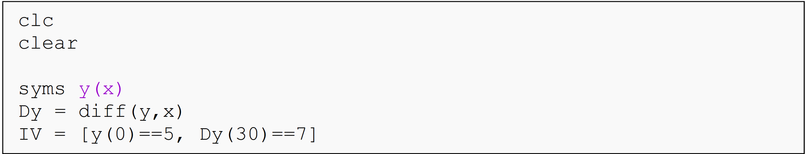
(a) dsolve(diff(y,x,2) == 5*x*(30-x), IV, x)

(b) dsolve(diff(y,x,2) == 5*x*(30-x), IV, 'y')

(d) dsolve(D2y == 5*x*(30-x), IV)

(5). A MATLAB function that finds the numerical solution to an ordinary differential equation is

(a) ode45()

(b) oda555()

(d) trapz()

Problem Set

(1). Solve the following initial value differential equation in MATLAB. \[\displaystyle3\frac{dy}{dx} + 6y = e^{- x}, \ \ y(0) = 6\].

Find \(y(10)\).

(2). Solve the following initial value differential equation in MATLAB.

\[\displaystyle7\frac{d^{2}y}{dx^{2}} + 11\frac{dy}{dx} + 13y = \sin(x), \ \ y(0) = 6, \ \ y'(0) = 17\]

Find \(y(10)\) and \(y'(10)\). Plot \(y\) as a function \(x\)from \(x =0\) to \(x=20\).

(3). Solve the following boundary value differential equation in MATLAB.

\[\frac{d^{2}y}{dx^{2}} - 3 \times 10^{- 6}y = 7.5 \times 10^{- 7}(100 - x), \ \ y(0) = 0, \ \ y(100) = 0\]

Find \(y(15)\), and the maximum value of \(y\).

(4). A ball bearing at \(1200K\) is allowed to cool down in air at an ambient temperature of \(300K\). Assuming heat is lost only due to radiation, the differential equation for the temperature of the ball is given by

\[\displaystyle\frac{d\theta}{dt} = - 2.2067 \times 10^{- 12}\left( \theta^{4} - 81 \times 10^{8} \right), \ \ \theta(0) = 1200K\]

where \(\theta\) is in \(K\) and \(t\) in seconds. Using MATLAB, find the temperature, the rate of change of temperature, and the rate at which heat is lost at \(t = 480\) seconds. The rate at which the heat is lost (in Watts) is given by

\[\text{Rate at which heat is lost} = 2.42 \times \text{1}\text{0}^{- 10}\ (\theta^{4} - 81 \times 10^{8})\]

(5). Pollution in lakes can be a serious issue as they are used for recreational use. One is generally interested in knowing that if the concentration of a particular pollutant is above acceptable levels. The differential equation governing the concentration of pollution in a lake as a function of time is given by

\[25 \times 10^{6}\frac{dC}{dt} + 1.5 \times 10^{6}C = 0\]

If the initial concentration of the pollutant is \(10^{7}\text{parts}/m^{3}\), and the acceptable level is \(5 \times 10^{6}\text{parts}/m^{3}\), how long will it take for the pollution level to decrease to an acceptable level? Plot the concentration of the pollutant as a function of time from the initial time to the time it takes the pollution level to decrease to the acceptable level.

(6). The speed (rad/s) of a motor without damping for a voltage input of 20 V is given by

\[\displaystyle20 = (\text{0.02})\ \frac{dw}{dt} + (0.06)w\]

If the initial speed is zero \(\displaystyle(w(0)=0)\) , what is the speed of the motor at \(t = 0.8s\)? What is the angular acceleration of the motor at \(t = 0.8s\).

(7). For a solid steel shaft to be shrunk-fit into a hollow hub, the solid shaft needs to be contracted. Initially at a room temperature of \(27\ ^{o}C\), the solid shaft is placed in a refrigerated chamber that is maintained at \(- 33\ ^{o}C\). The differential equation governing the change of temperature of the solid shaft \(\theta\) is given by

\[\displaystyle\frac{d\theta}{dt} = - 5.33 \times 10^{- 6}\begin{pmatrix} - 3.69 \times 10^{- 6}\theta^{4} + 2.33 \times 10^{- 5}\theta^{3} + 1.35 \times 10^{- 3}\theta^{2} \\ + 5.42 \times 10^{- 2}\theta + 5.588 \\ \end{pmatrix}(\theta + 33)\]

Using MATLAB, find the temperature and the rate of change of temperature after the steel shaft has been in the chamber for 12 hours.