Module 8: Loops
Learning Objectives
After reading this lesson, you should be able to:
reference matrices inside a loop,
store multiple values in a matrix,
access specific portions of a matrix such as the diagonal or the upper triangle,
identify a special matrix.
This lesson combines several pieces of programming knowledge you have learned and used so far including matrices (Lesson 2.6), conditional statements (Module 5), and nested loops (Lesson 8.4) in MATLAB. In this lesson, you will see some of the nuances and tricks associated with using matrices in loops.
How can I reference matrices in a loop?
As noted in several previous lessons, a vector is a special type of
matrix: a one-dimensional matrix. Everything said about matrices in this
lesson will also (generally) apply to vectors. Also, recall vectors and
matrices as mathematical concepts that were covered in Lesson 4.6 as
well as the common MATLAB functions relating to these concepts such as
size(). We will
start by showing examples for referencing both a vector and a matrix in
a loop just to be clear.
In this module, we also talked about running a block of code multiple times using loops. In the case of arrays (vectors and matrices), this is useful when referencing many different elements stored inside them: the less “automatic” alternative is referencing every array element manually.
Referencing an array typically means calling out a specific subset of
that array. For example, given vec = [3 7 5.4 8 9], we could reference
the first three elements with vec(1:3). The values giving the location
(e.g., the first and second elements) of the desired elements are often
called the index/indices. However, it is common to need to reference
each element of a given vector. To do this, we need to use loops.
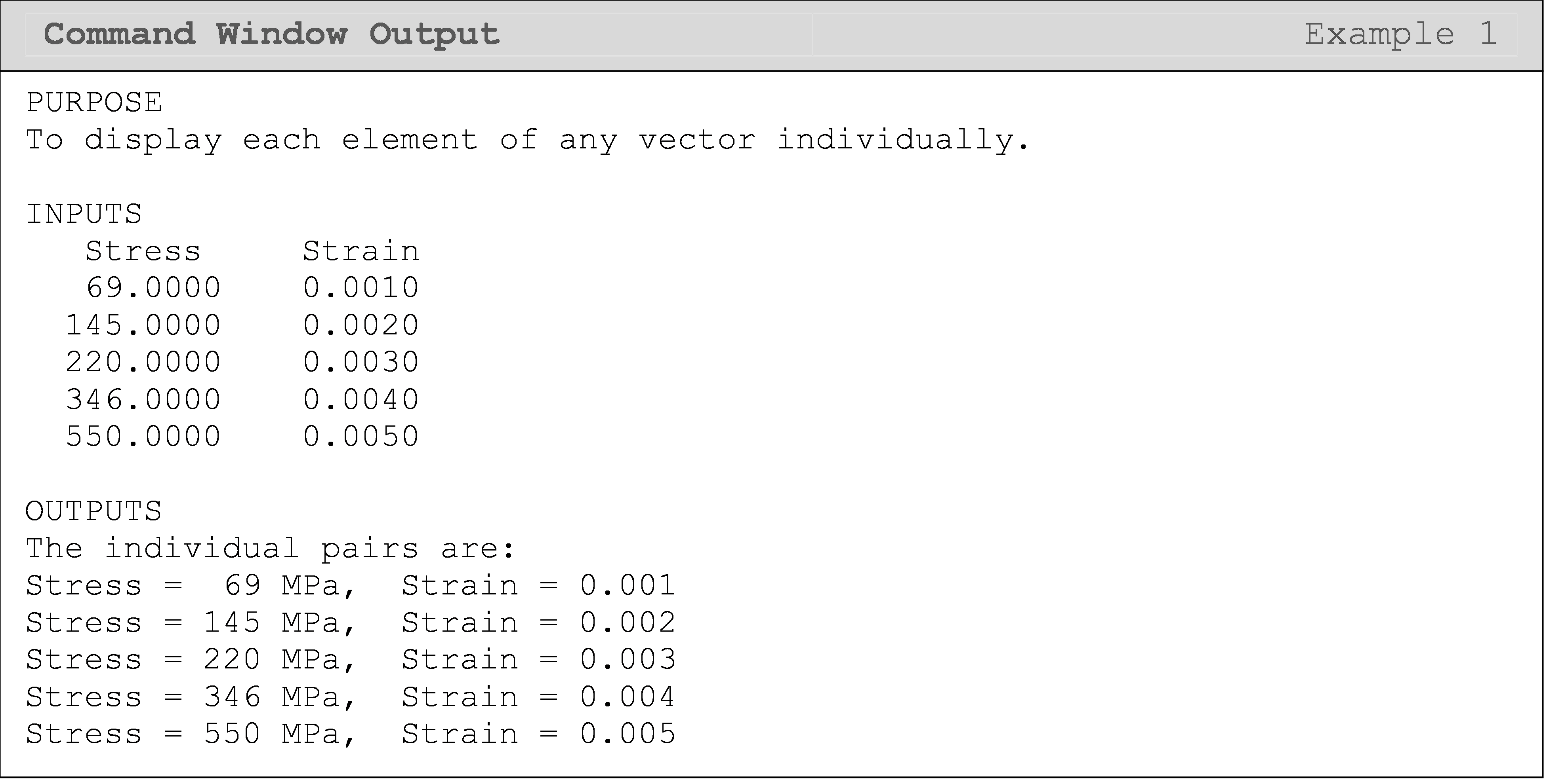
Example 1
Consider the data given in Table 1 that was collected during axial testing of a metal specimen. In this test, the value of stress and strain is measured at various stages of the experiment. We know we can find Young’s modulus of the metal by finding the relationship between stress and strain.
Table 1: Stress vs. Strain data of a material.
| Strain | Stress (MPa) |
|---|---|
| 0.001 | 69 |
| 0.002 | 145 |
| 0.003 | 220 |
| 0.004 | 346 |
| 0.005 | 550 |
Any element of a vector can be individually “called” for further analysis by using matrix parenthesis notation as discussed above and in Lesson 2.6. Using the same parenthesis notation, a loop can be written to display each stress measurement with the corresponding strain measurement.
Write a program that displays each set of corresponding stress and strain elements in the Command Window.
Solution

The two vectors of stress and strain can now be used to generate a stress vs. strain plot, and to find Young’s modulus of the metal (see problem 4 of the exercise set of this exercise).
At this point, one might ask, “Why don’t we just do disp(stress)?” This
would not display each element individually. “Well, why not
disp(stress(1)), disp(stress(2)), …” This would not address the
“any” part of the question. The solution should work for any given
vector, which means for any given length (number of elements). So, if
you wrote code in that form for a vector with six elements and then
tried to use that code on a vector with four elements, MATLAB would
return an error. If you used that code on a vector with eight elements,
you would get only six out of the eight elements You should try this for
yourself using the solution from Example 1.
Notice that we can reference a vector with a single loop since one of
the dimensions will be held at 1. That is, vec(i,1) and vec(i) are
equivalent programming references and evidently only require one
iterating (changing) variable in a loop.
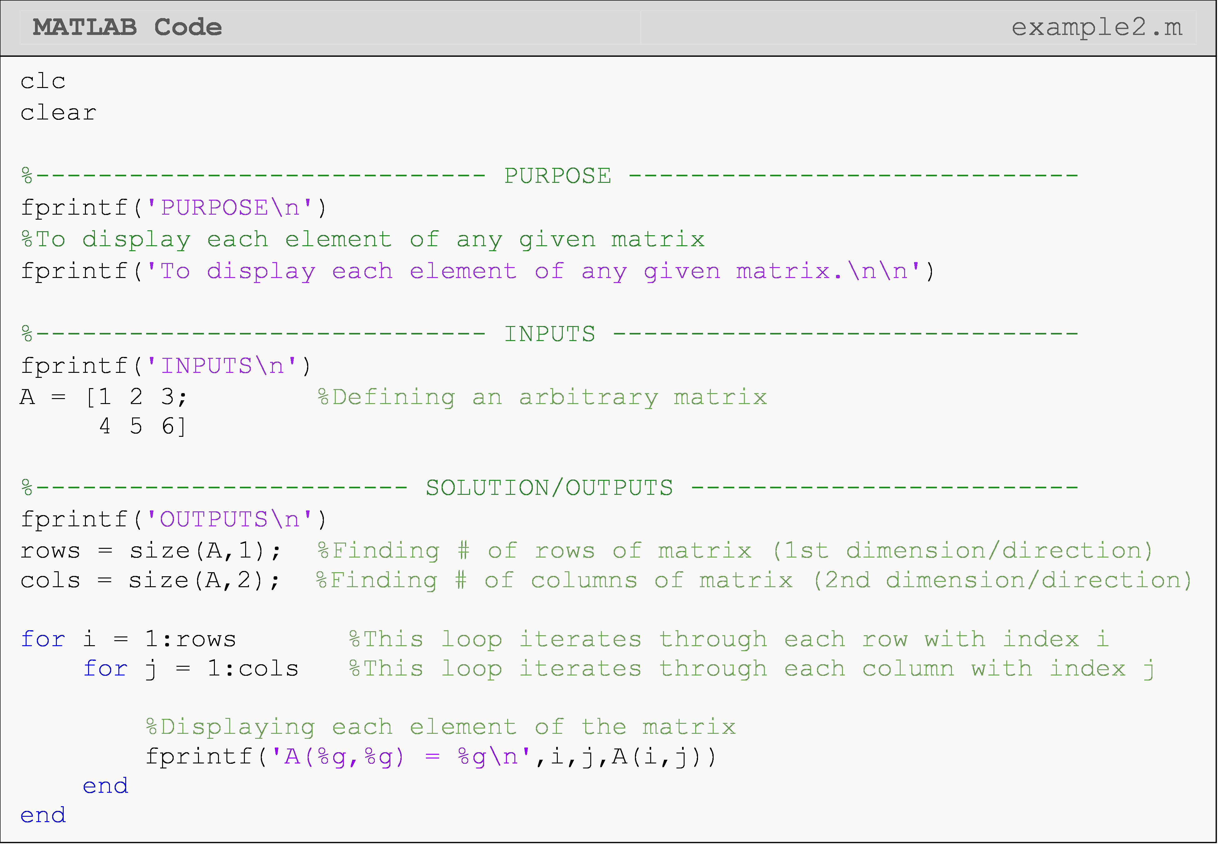
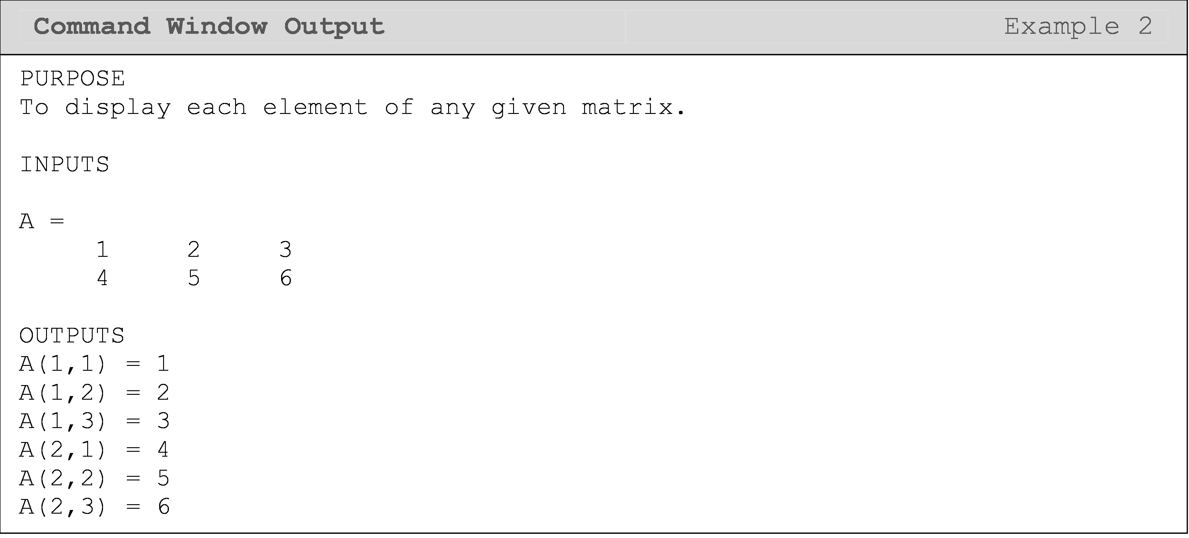
In the next example, which uses a matrix, we will need two loops. Perhaps you can guess that it is because both the rows and the columns will need iterators (changing variables). Also, note that we want to “look at” or reference one column or one row of the matrix per loop iteration. Therefore, we will use a nested loop where the parent/outer loop remains constant, while the nested/inner loop runs from the beginning to the- end. In Example 2, this has the effect of looking at an entire row of the matrix before moving on to the next row. Look at the outputs to verify this for yourself!
How do I store values in a matrix using a loop?
Often, it is useful to store values obtained in each loop, so you have a vector or matrix of values at the end of the loop(s). While in the previous example we referenced values/elements in an existing matrix, here we create a matrix element-by-element. Figure 1 shows a generalized visualization for storing in a vector, and Example 3 shows a code that stores values in a vector.
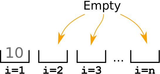
Figure 1: A visualization of the process for generating a vector.
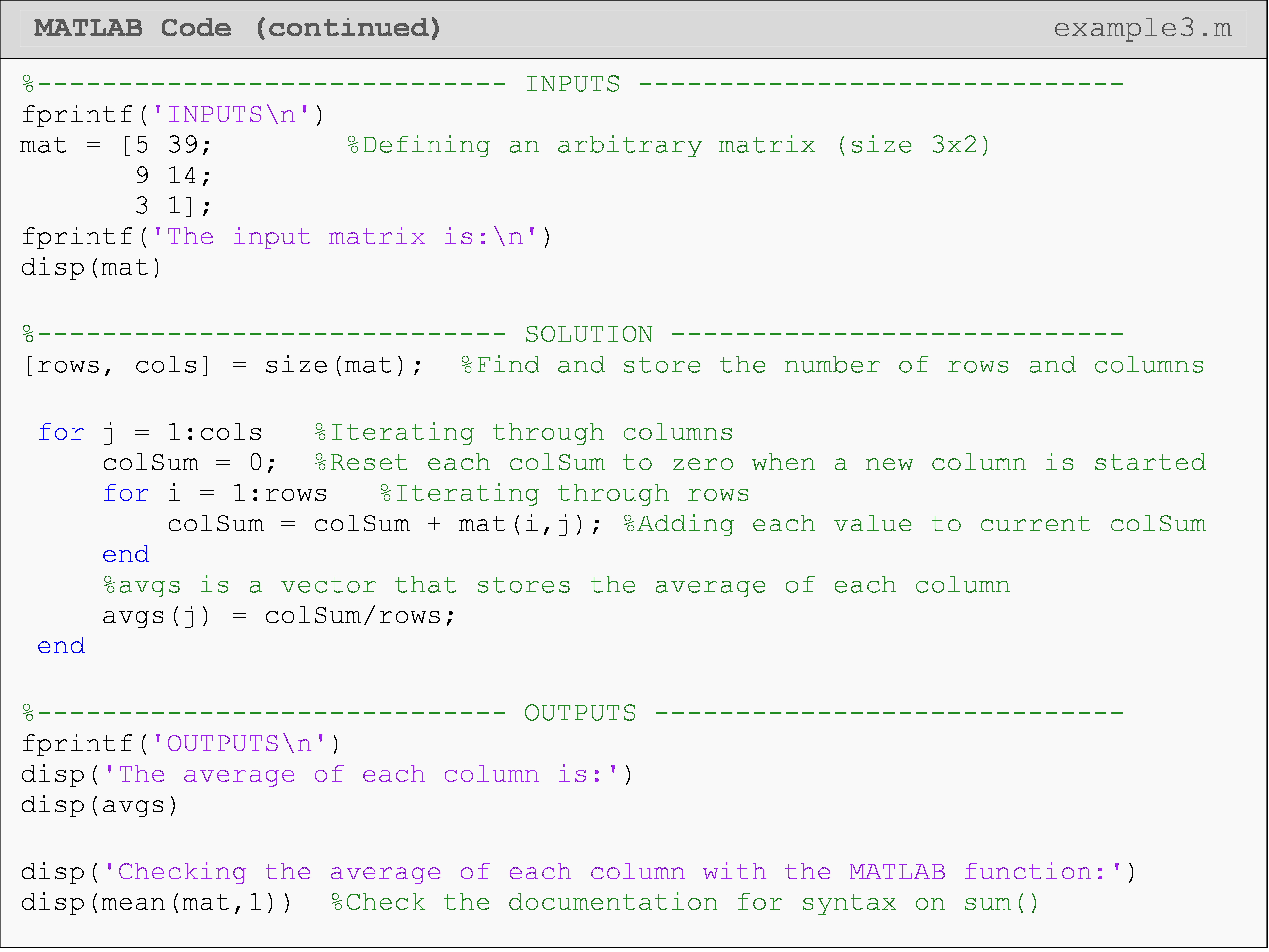
As discussed earlier in this lesson, the outer loop remains constant for one entire completion of the inner loop. We will take advantage of this behavior in Example 3 where we want to average the numbers in each column. Therefore, we want to hold the column number constant (parent loop) while we loop through all the rows of that column with the nested loop. This means that we will go through (average) all the elements in the first column, then the second, and so on.
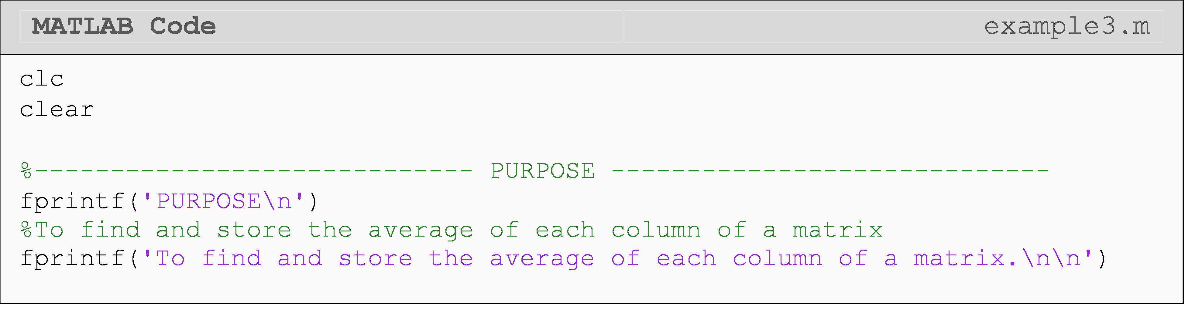
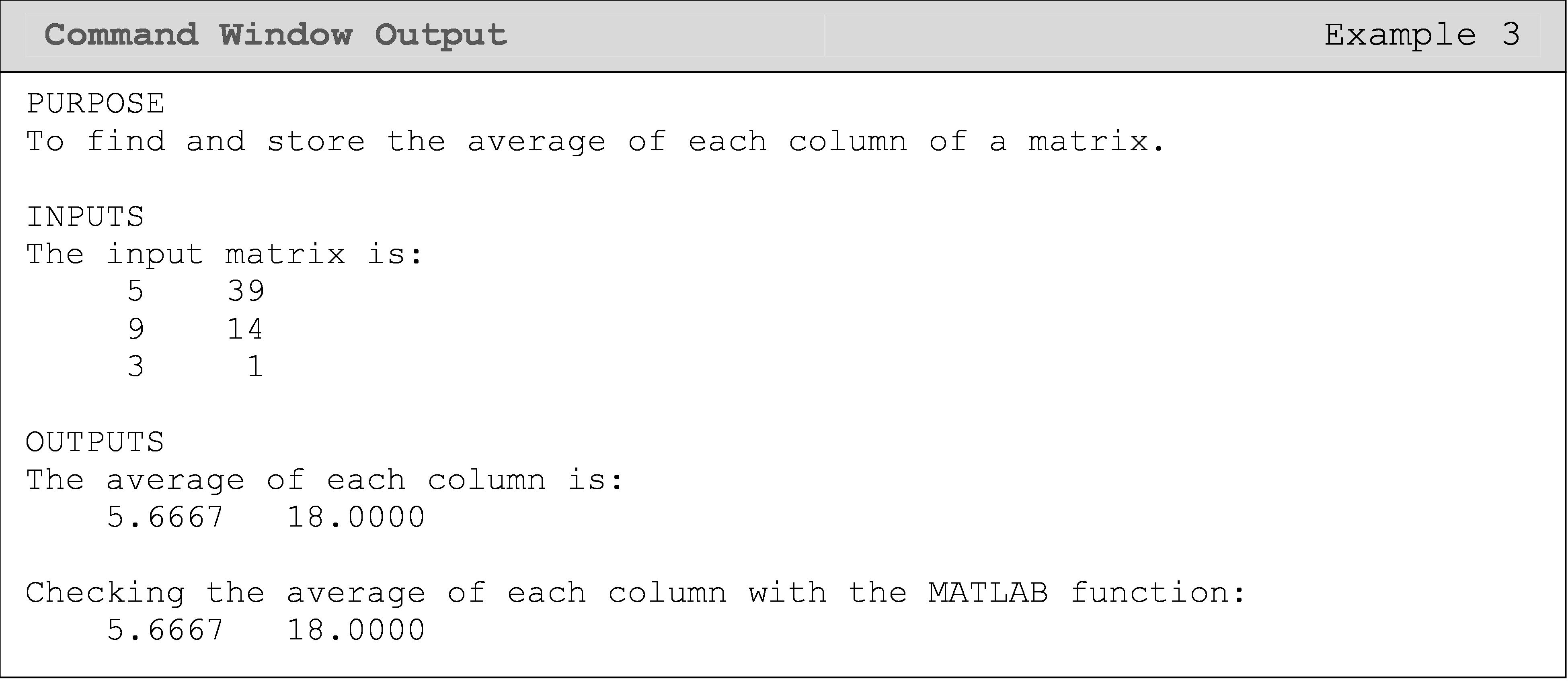
Example 3
Find the average of each column in any given matrix without using use
the built-in functions such as mean() and sum(). Store the averages in a
vector and display the final vector of averages in the Command Window.
Use the matrix given below as a test case.
\[[B] = \displaystyle \begin{bmatrix} \text{5} & \text{39} \\ \text{9} & \text{14} \\ \text{3} & \text{1} \\ \end{bmatrix}\]
Solution
Another real-world example would be if you have a line of code that gets the pressure inside a tank each time the function is run. However, you want to plot and analyze this data changing over time. To do this, you will need to run the sensor read code many times with a loop, and each time the loop runs (the sensor is read), you will need to store that reading in a vector or matrix (depending on how many values are returned by the sensor).
How can I access specific areas of a matrix?
It is useful to understand how to write conditions to reference different parts of a matrix such as upper triangular, lower triangular, and diagonal portions. These three conditions are shown visually in Figure 2. To find these or other locations yourself, just write down the matrix elements, A(i,j), for the area of the matrix you want to reference and look for a pattern. For example, to find the condition for all diagonal elements, just write out A(1,1), A(2,2), A(3,3), A(4,4). You can immediately see diagonal elements always occur when \({i} = {j}\).
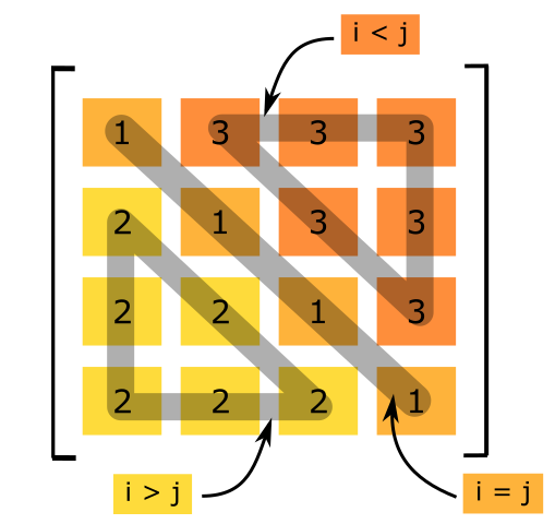
Figure 2: Shows conditions to reference different portions of a
matrix.
Examples 4 further demonstrates how to access different locations in a
matrix. It also demonstrates how to create a matrix element-by-element,
which is just another way of “storing” values. This is a very common
task when programming, and therefore, it is essential to fully
comprehend. Although the difference of “storing” versus “referencing”
may still be foreign, just remember to check which side (left or right)
the equals operator (=) the variable in question is on. This will always
tell you whether the variable is being referenced or assigned a value
(something is being stored in the variable).
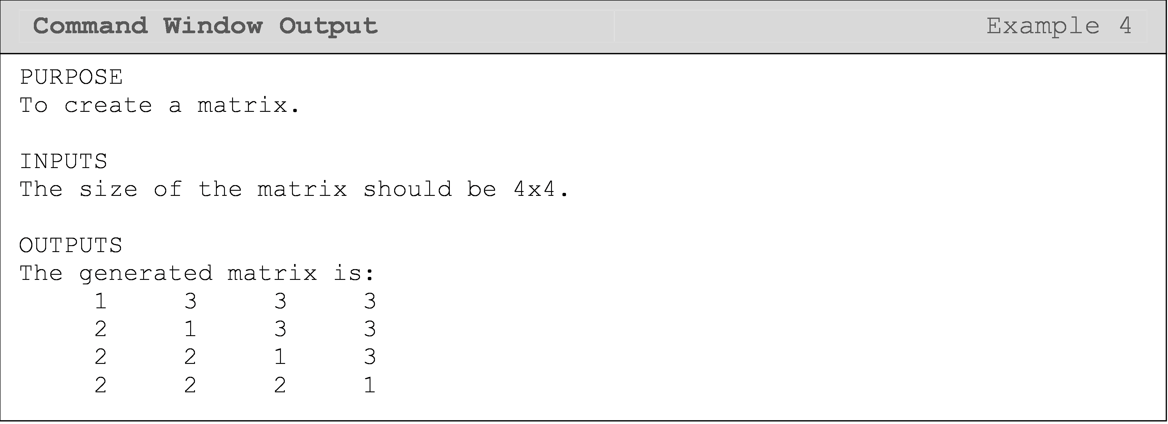
Example 4
Write a code that creates a square matrix of the same form like the one shown in Figure 2. The only input is the size of the square matrix.
Solution
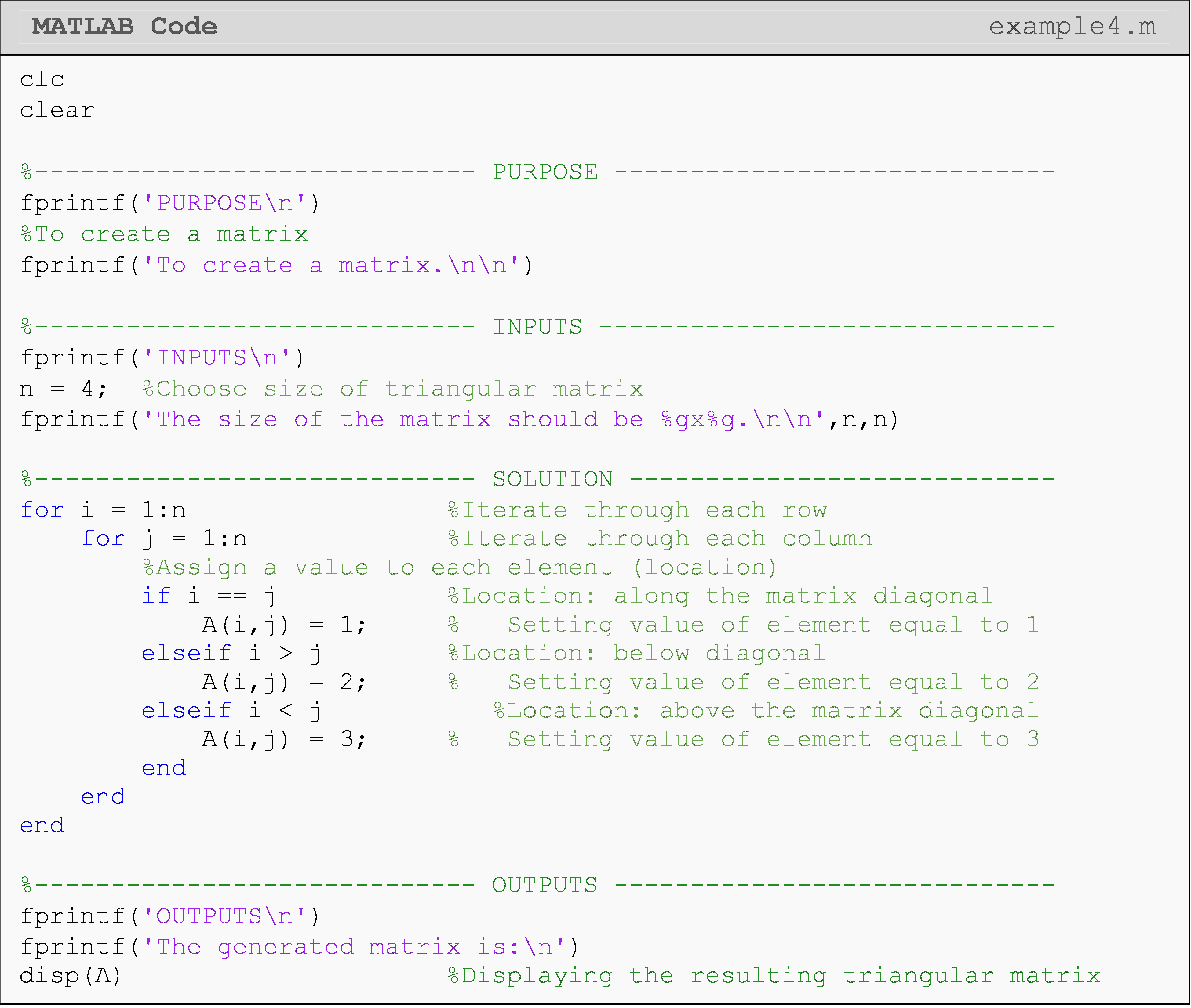
Notice we need two loops to access every element in a matrix: one loop for each matrix direction. For vectors, we needed only one loop to access each element. As you will see in Lesson 8.7 with the sorting example, having a vector as an input does not always mean you need only one loop. You need at least one loop to access (or “look at”) each element of a vector individually, but depending on the problem, you may need more. A similar statement is true for matrices. One notable, special case is when one only needs to access the diagonal of a matrix. One such application is shown in Example 5.
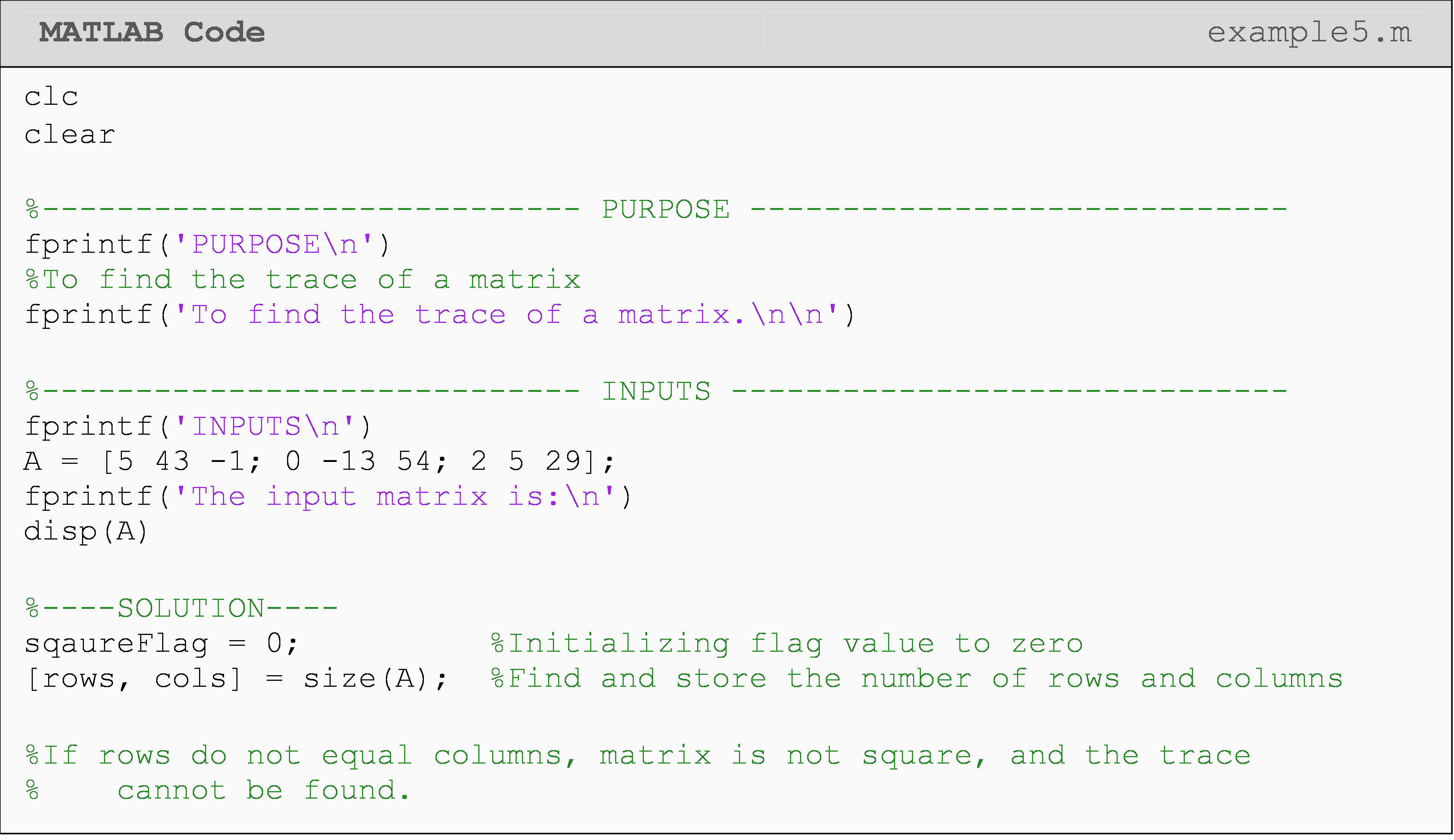
Example 5
The trace of a matrix is defined only for a square matrix (that is, the number of rows is the same as the number of columns) and is the summation of all its diagonal elements. For a square matrix [A] of size \(n \times n\), the trace of a matrix [A] is given by
\[ [A]= \displaystyle\sum_{i=1}^n a_n\]
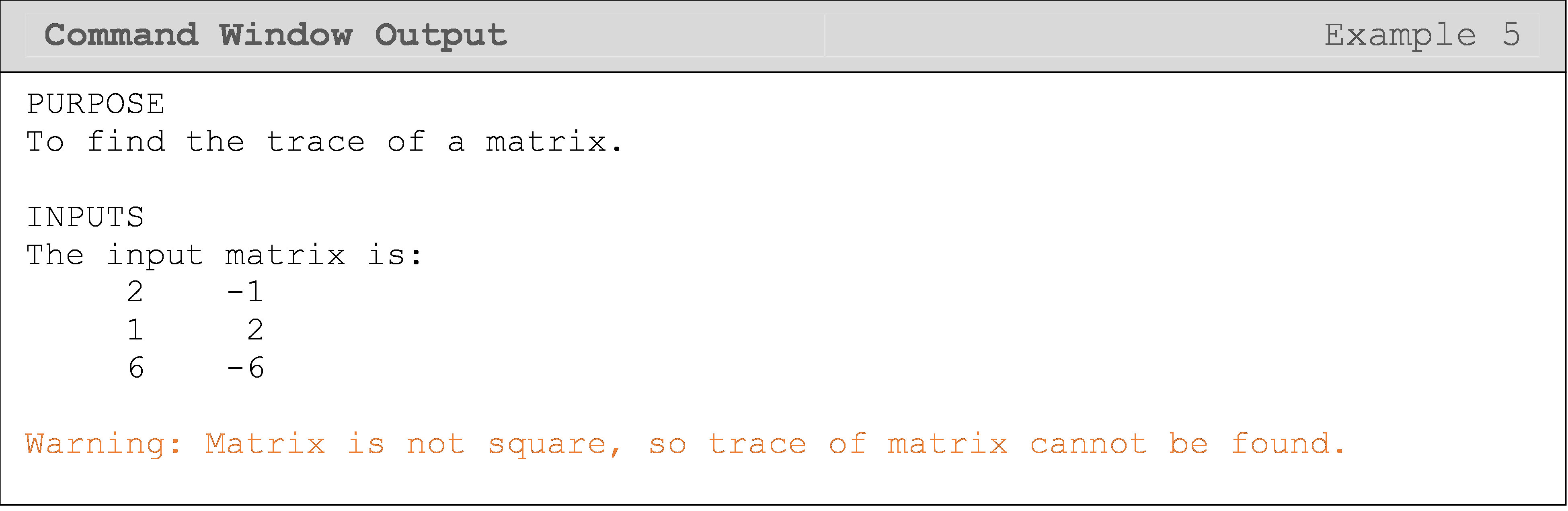
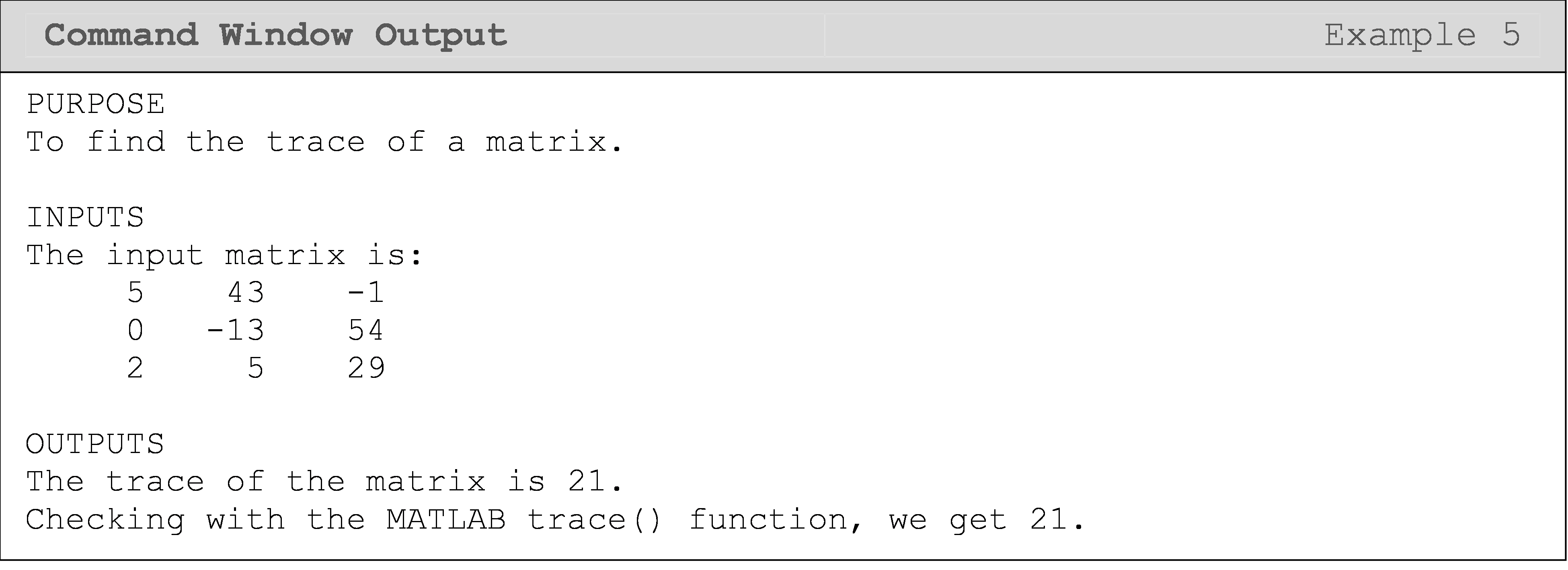
Find the trace of any square matrix. The program must also automatically test if the matrix is square.
Test the program with the following two matrices [A] and [B]:
\([A]=\begin{bmatrix} 2 & -1\\ 1 & 2\\ 6 & -6 \end{bmatrix}\) \([B]=\begin{bmatrix} 5 & 43 & -1\\ 0 & -13 & 54\\ 2 & 5 & 29 \end{bmatrix}\)
Solution
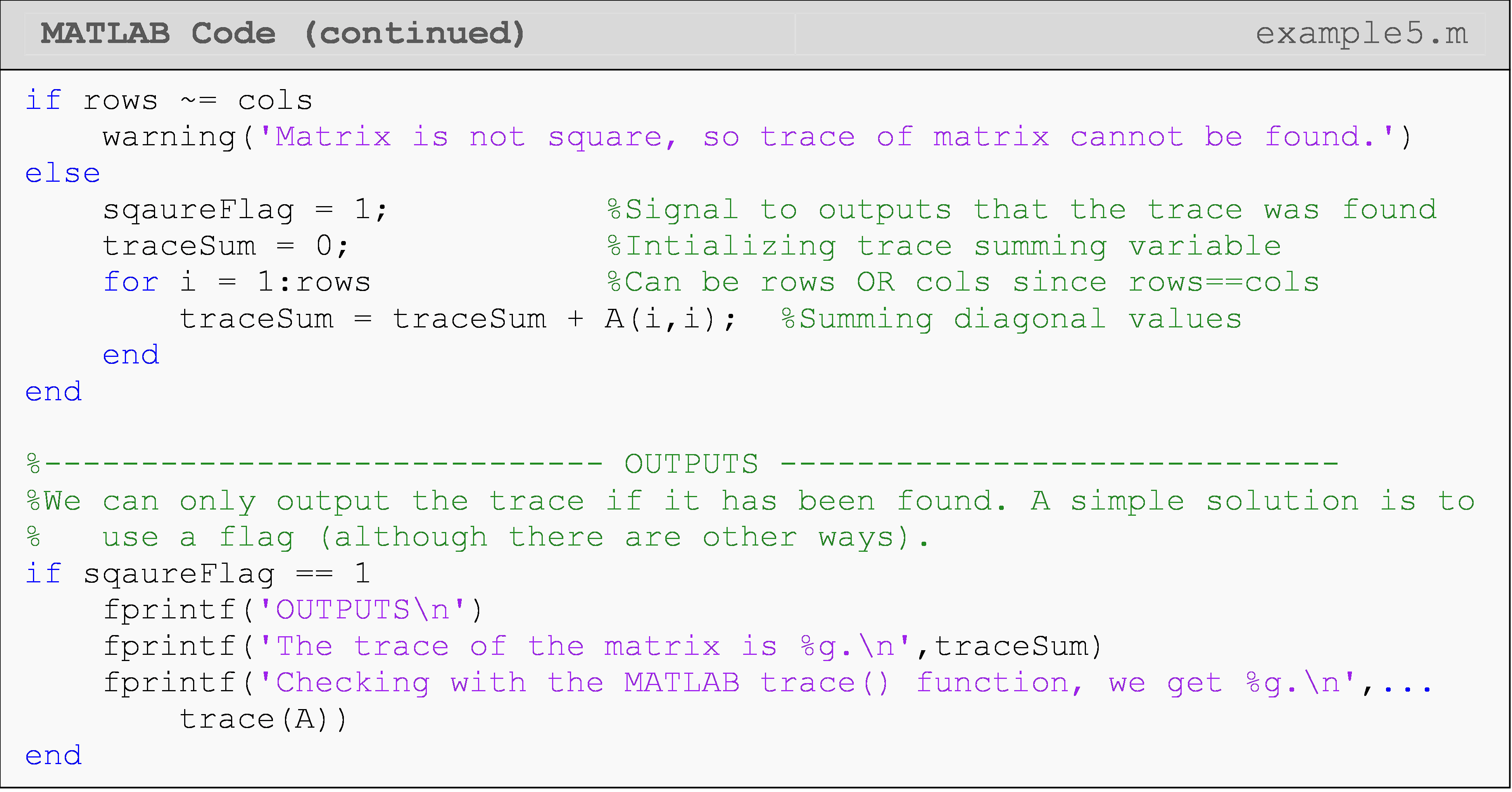
The following Command Window outputs are shown for different matrix inputs. Notice the first Command Window shown has a non-square matrix, which yields an error, while the second Command Window output shown is for a square matrix input.
We can use what we have learned so far in this lesson to test for a specific type of matrix (Example 6). The only extra information one needs to know in these cases is the definition of that special type of matrix, which has little to do with programming skills.
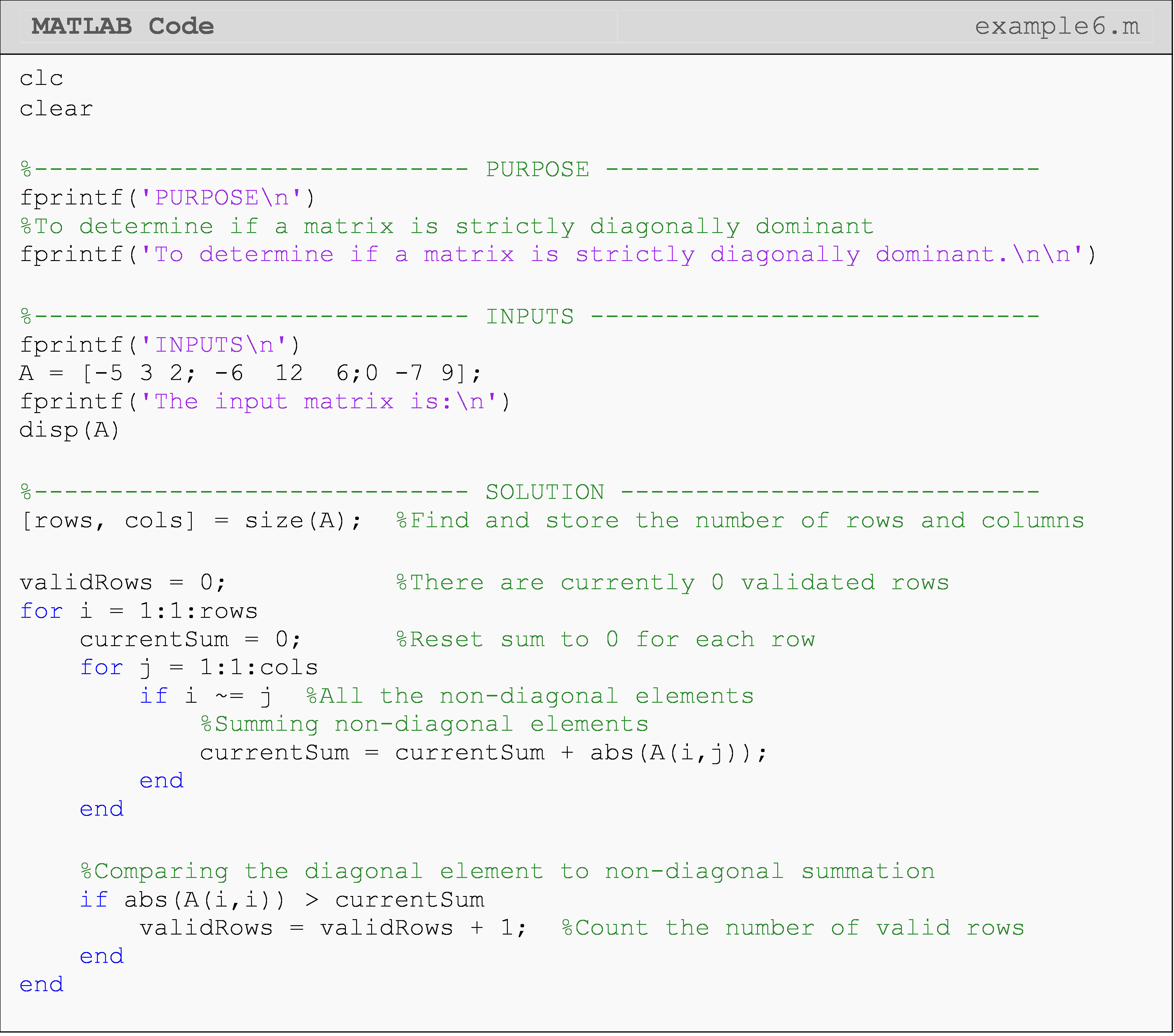
Example 6
Many a time, it is efficient to solve a set of simultaneous linear equations by using iterative schemes such as Gauss-Seidel method. In such cases, the convergence of the solution is guaranteed if the coefficient matrix is strictly diagonally dominant.
To determine if a square matrix is strictly diagonally dominant or not, one compares the row diagonal element to the row non-diagonal elements. For each row, the absolute value of the diagonal element must be strictly greater than the sum of the absolute value of the non-diagonal terms. If this condition is true for all rows, only then the matrix is strictly diagonally dominant (SDDM).
Mathematically, a square matrix [A] of \(n \times n\) size can be defined as strictly diagonally dominant if
\[|a_{ij}|>\sum_{\begin{matrix}j=1\\ i \neq j\end{matrix}}^{n} |a_{ij}| \ \ \ \text{for } i =1, 2, ... , n.\]
Take the following matrix as an example
\[ [S]=\begin{bmatrix} -5 & 1 & 2\\ -6 & 12 & 3\\ 1 & -7 & 9 \end{bmatrix}\]
This is a strictly diagonally dominant matrix because all the rows meet the criteria as shown below.
\[\begin{split} |-5|&>|1|+|2|\\ 5&>3\\ |12|&>|-6+|3|\\ 12&>9\\ |9|&>|1|+|-7|\\ 9&>8 \end{split}\]
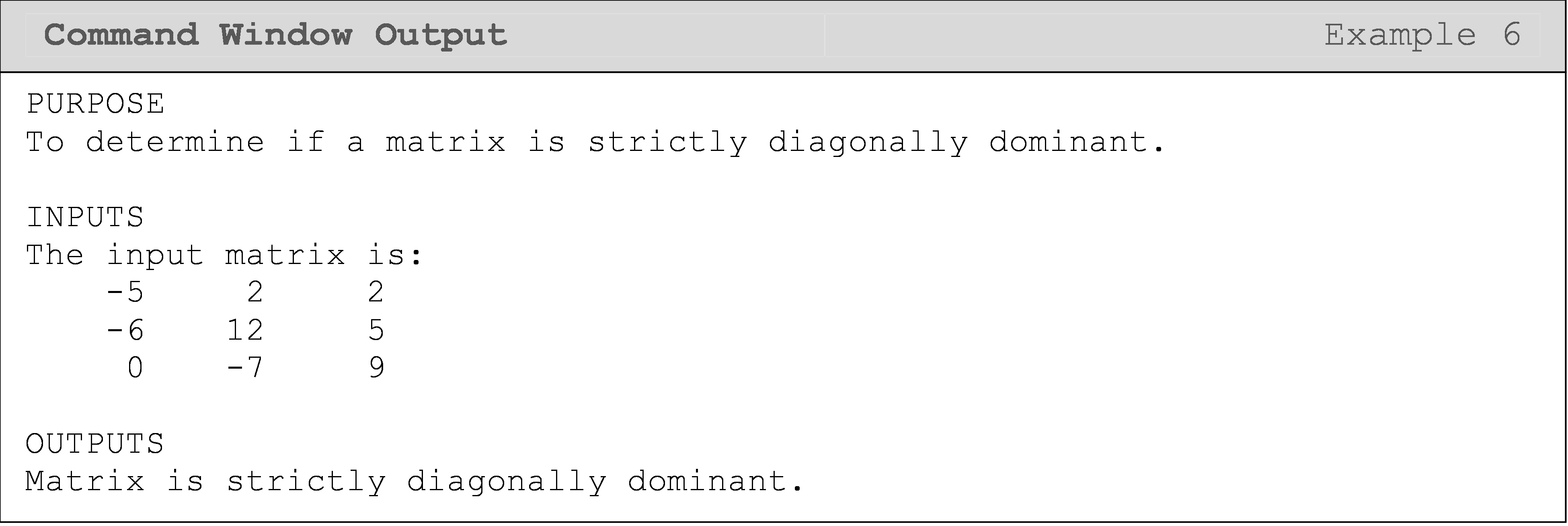
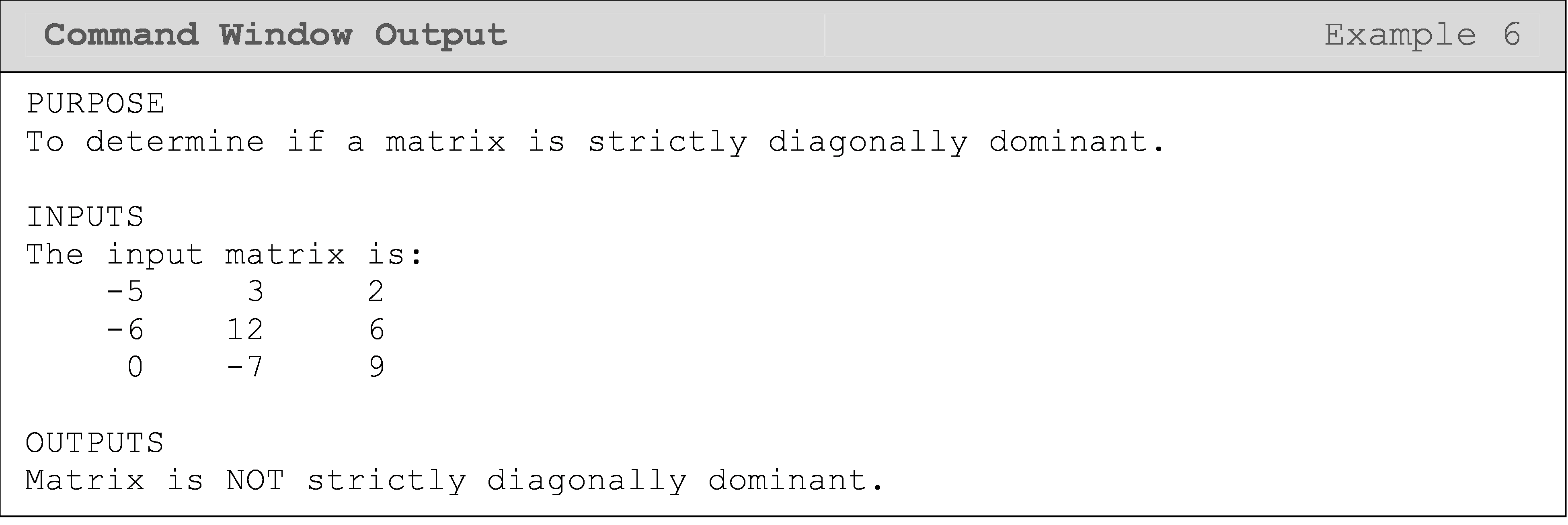
Write a program that determines if a square matrix is strictly diagonally dominant (SDDM) or not.
Test the program using the following two matrices, [A] and [B].
\([A]=\begin{bmatrix} -5 & 2 & 2\\ -6 & 12 & 5\\ 0 & -7 & 9 \end{bmatrix}\) \([B]=\begin{bmatrix} -5 & 3 & 2\\ -6 & 12 & 6\\ 0 & -7 & 9 \end{bmatrix}\)
Solution
We need two loops to access each element in the matrix. An if statement
is used within the nested loop to sum only the non-diagonal elements.
Finally, the current row non-diagonal sum is compared to the row
diagonal element. If it meets the criteria, it is added to the validRows
count. This is done in the parent loop (i) because the diagonal elements
can be referenced with only one loop. Therefore, placing this code
inside the nested loop (j) would needlessly repeat the code and make the
program less efficient.
If at the end of the loops, the number in the validRows variable is
equal to the number of rows of the matrix, then the condition of the
matrix being an SDDM is met.
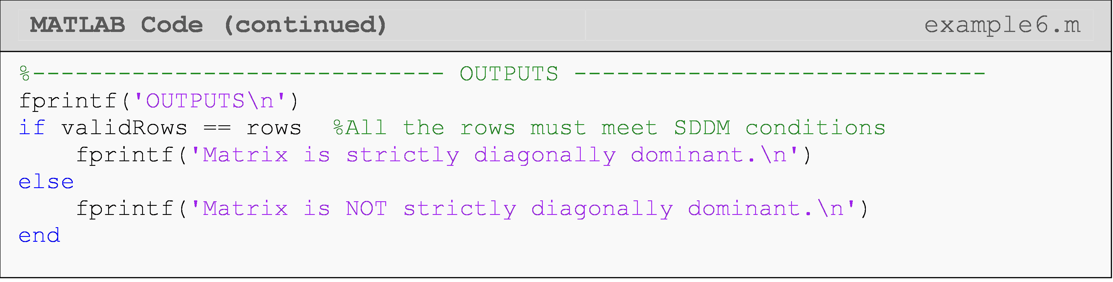
The following Command Window outputs are shown for different matrix inputs. As you can see, the first matrix input is strictly diagonally dominant, while the second is not.
What is vectorization?
Although it can be a good exercise to perform matrix operations like addition, subtraction, and multiplication the “long way” (i.e., the non-vectorized way) when first learning to use loops and work with matrices, it is not standard practice.
Vectorization is the practice of implementing elemental operations as matrix operations in programs. For example, if you have a system of three equations and three unknowns, you would vectorize the solution by putting the equations into matrix form, and find the solution using linear algebra. For many mathematical matrix operations, you should implement them in MATLAB using “vectorization” rather than loops as this takes advantage of the efficiency of MATLAB, and hence avoid unnecessary complexity in the code.
There are many examples where you can vectorize operations involving matrices in MATLAB. They include matrix addition, subtraction, and multiplication. More complex examples are when you combine these operations into equations. This occurs often in programming in areas like machine learning and state-space controls.
How can I vectorize matrix operations in MATLAB
The words “vectorize” and vectorization” may be new to you, but the concepts and syntax are not. Recall that Lesson 4.6 on Linear Algebra was where we first learned how to evaluate mathematical expressions and equations that contain matrices. We did not know anything about loops then, and therefore, the code we wrote was a vectorized solution! We did this for simple things like addition, subtraction, and multiplication of matrices as well as more complex tasks like solving systems of equations in matrix form. We recommend reviewing the examples from Lesson 4.6 to more fully grasp vectorization.
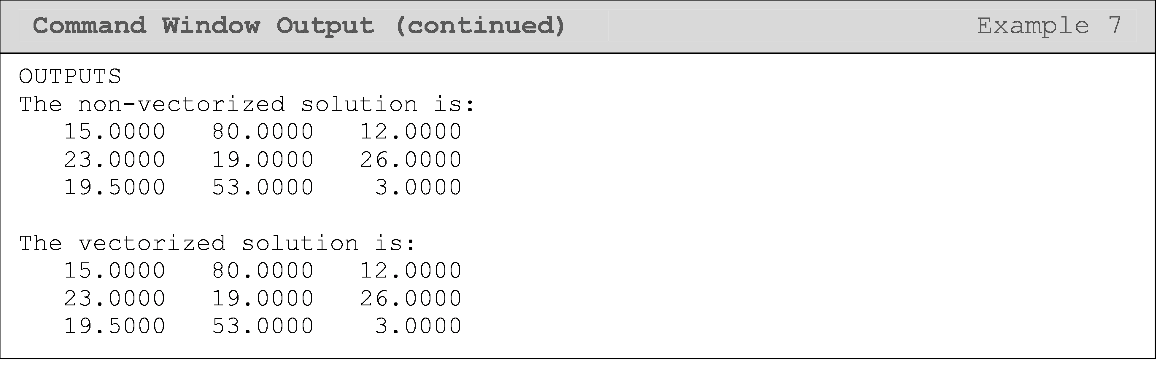
Examples 7 and 8 compare vectorized and non-vectorized solutions for matrix operations, which of course will return the same answers. Although it can be a good exercise to perform matrix operations like addition, subtraction, and multiplication the “long way” (i.e., the non-vectorized way) when first learning to use loops and work with matrices, it is not standard practice. When writing professional code, one should use vectorized solutions in MATLAB whenever possible. This is because it is the vectorized syntax that has been optimized to be faster than the equivalent element-by-element loop operations we could write.
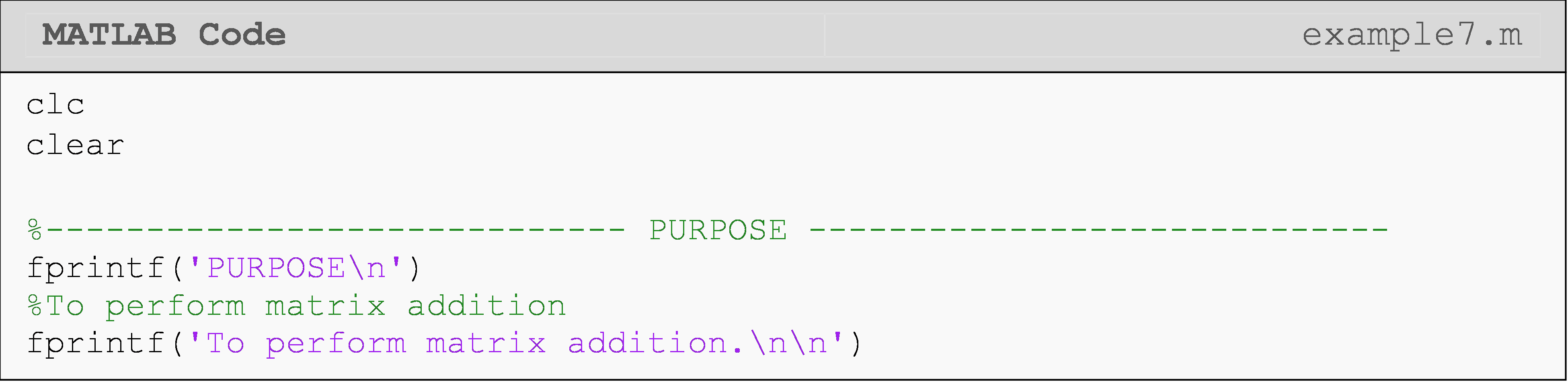
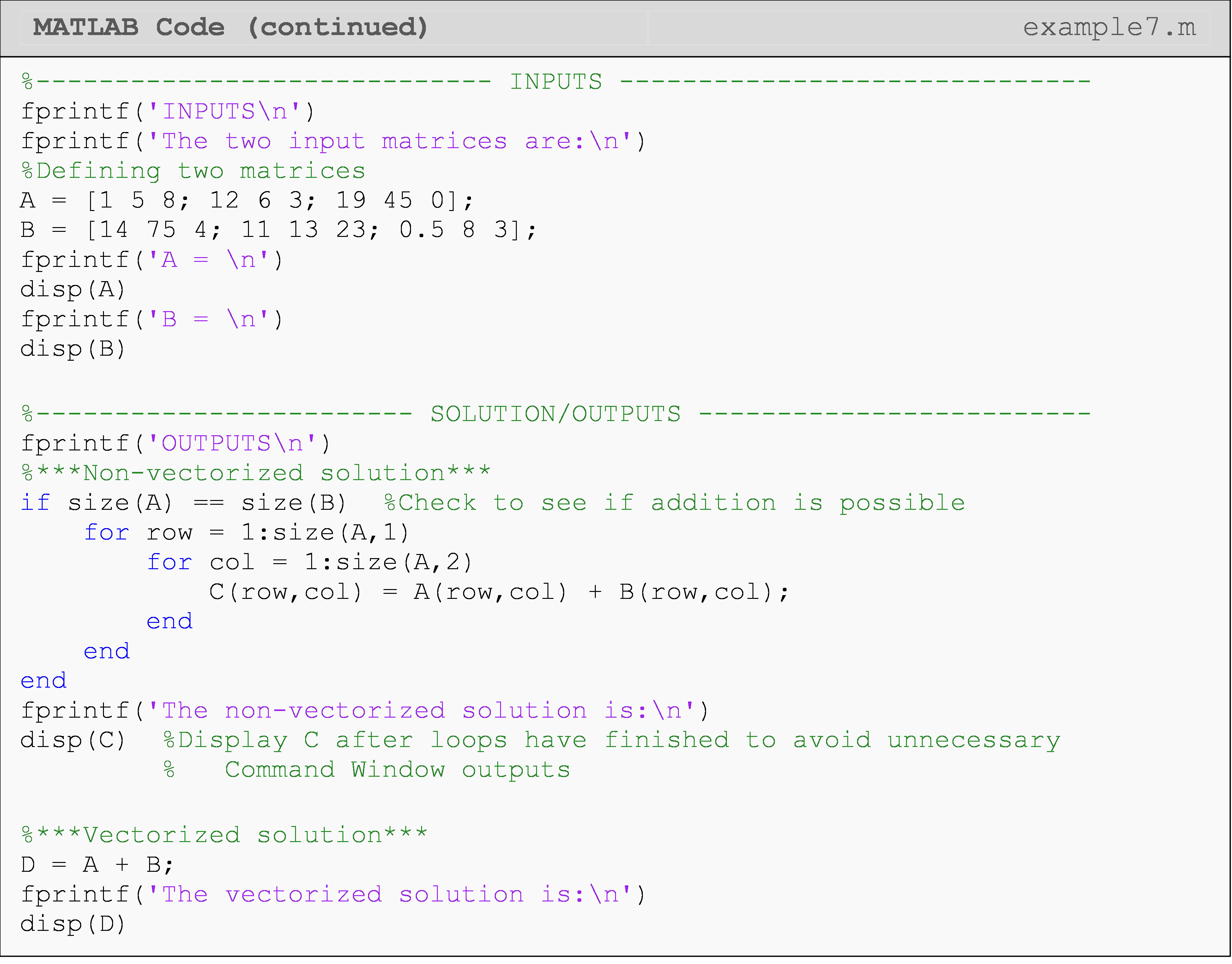
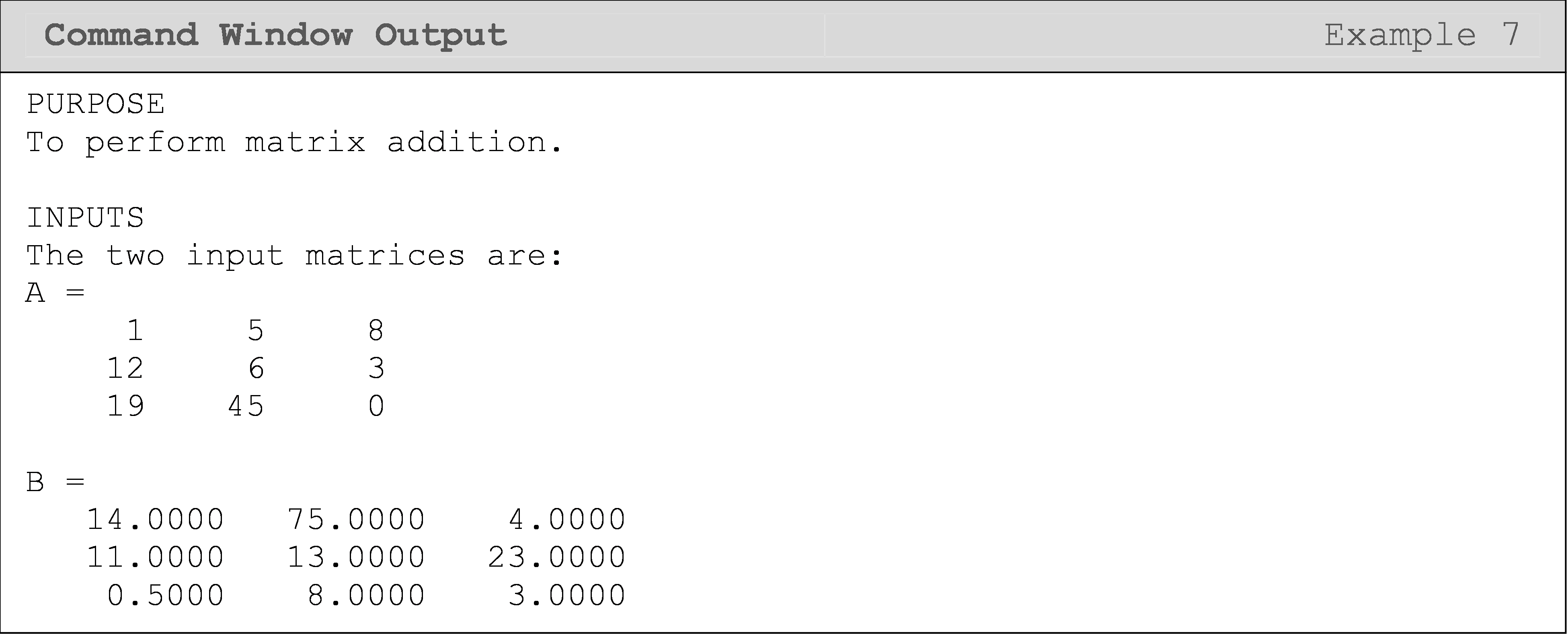
Example 7
Write a program that adds any two matrices (given that the matrices are of equal size) using element-by-element loops operations and vectorized operations. Use the matrices [A] and [B] to test your program.
\([A]=\begin{bmatrix} 1 & 5 & 8\\ 12 & 6 & 3\\ 19 & 45 & 0 \end{bmatrix}\) \([B]=\begin{bmatrix} 14 & 75 & 4\\ 11 & 13 & 23\\ 0.5 & 8 & 3 \end{bmatrix}\)
You should now be able to see why, in their documentation on vectorization, MATLAB lists the compactness of a vectorized matrix operation as improving the appearance of the code and reducing the complexity (and hence the likelihood of errors).
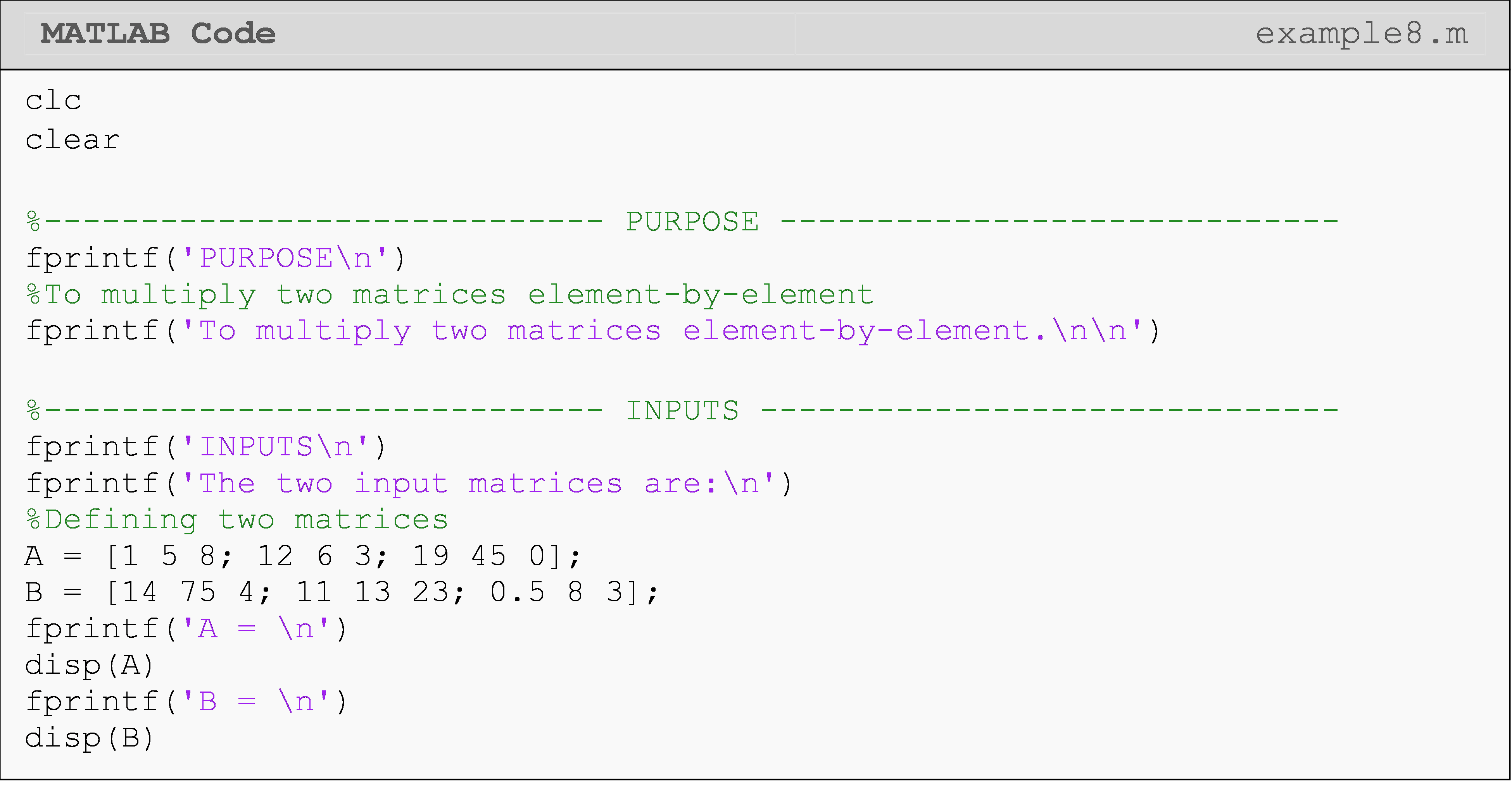
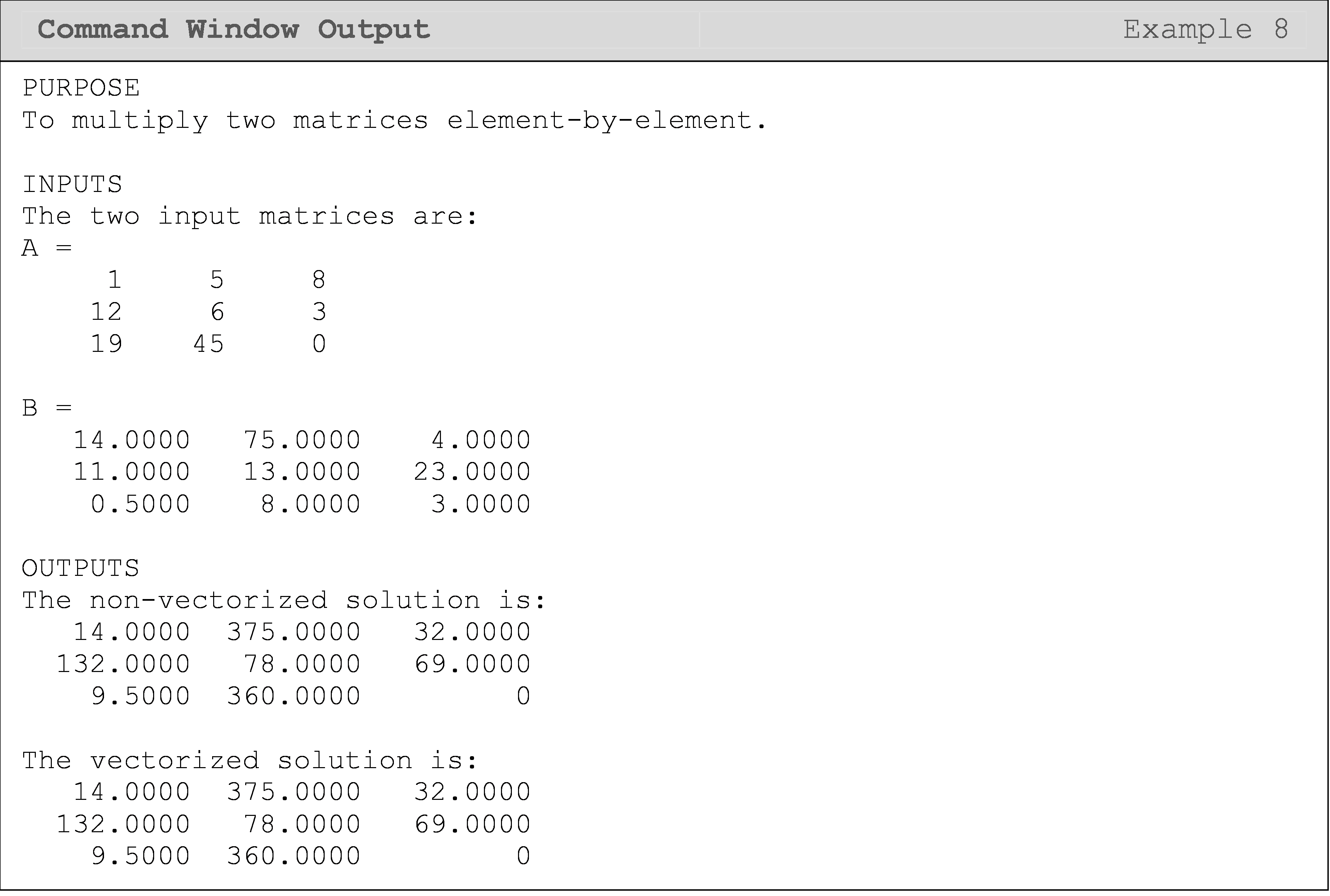
Example 8
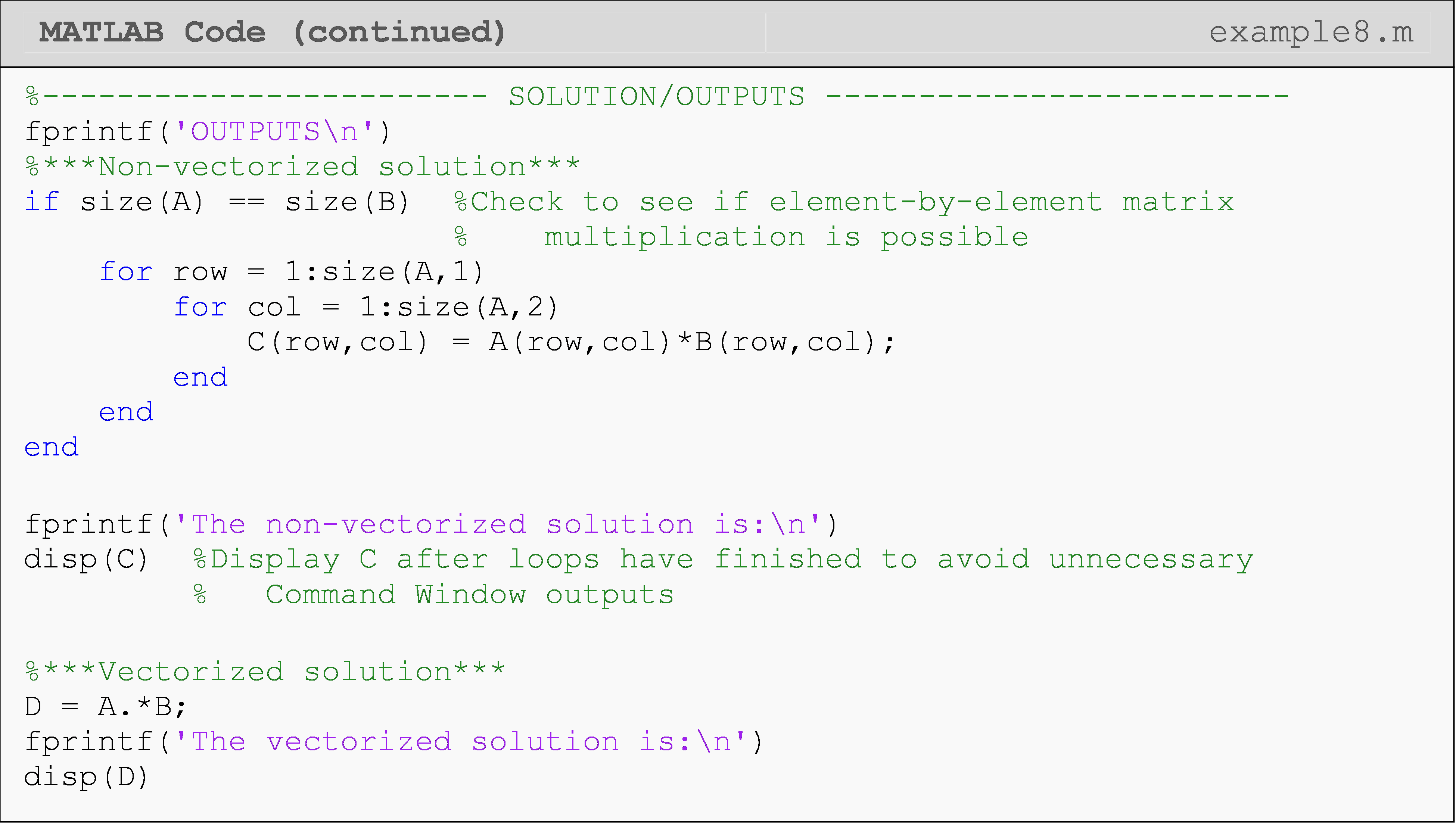
Write a program that finds the element-by-element product of any two square matrices of equal size using loops operations and vectorized operations. Use the matrices [A] and [B] to test your program.
\([A]=\begin{bmatrix} 1 & 5 & 8\\ 12 & 6 & 3\\ 19 & 45 & 0 \end{bmatrix}\) \([B]=\begin{bmatrix} 14 & 75 & 4\\ 11 & 13 & 23\\ 0.5 & 8 & 3 \end{bmatrix}\)
Solution
What are some tips I can use for vectorization?
Below are a few tips to keep in mind when you are trying to vectorize equations containing matrices/vectors.
Use short variable names for vectors and matrices when possible.
Be sure to know what you want to happen and what is happening during the evaluation (calculation) of your equations in MATLAB. This always applies to programming.
Make sure you understand and appropriately use array and matrix operations (common mistake).
Use the shorthand (') for the transpose of a matrix.
Multiple Choice Quiz
(1). The Command Window output of the following program is
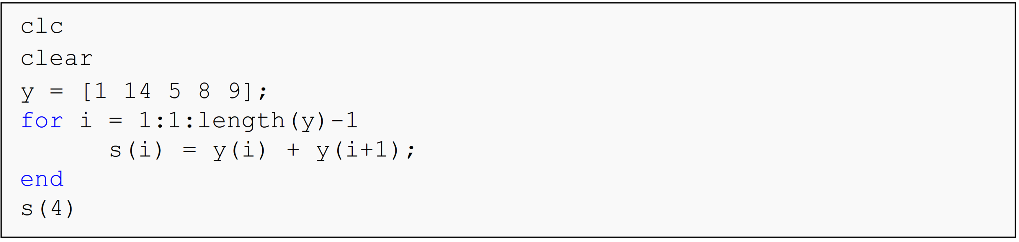
(a) ans = 17
(b) ans = 15
(c) ans = 13
(d) ans = 19
(2). The Command Window output of the following program is
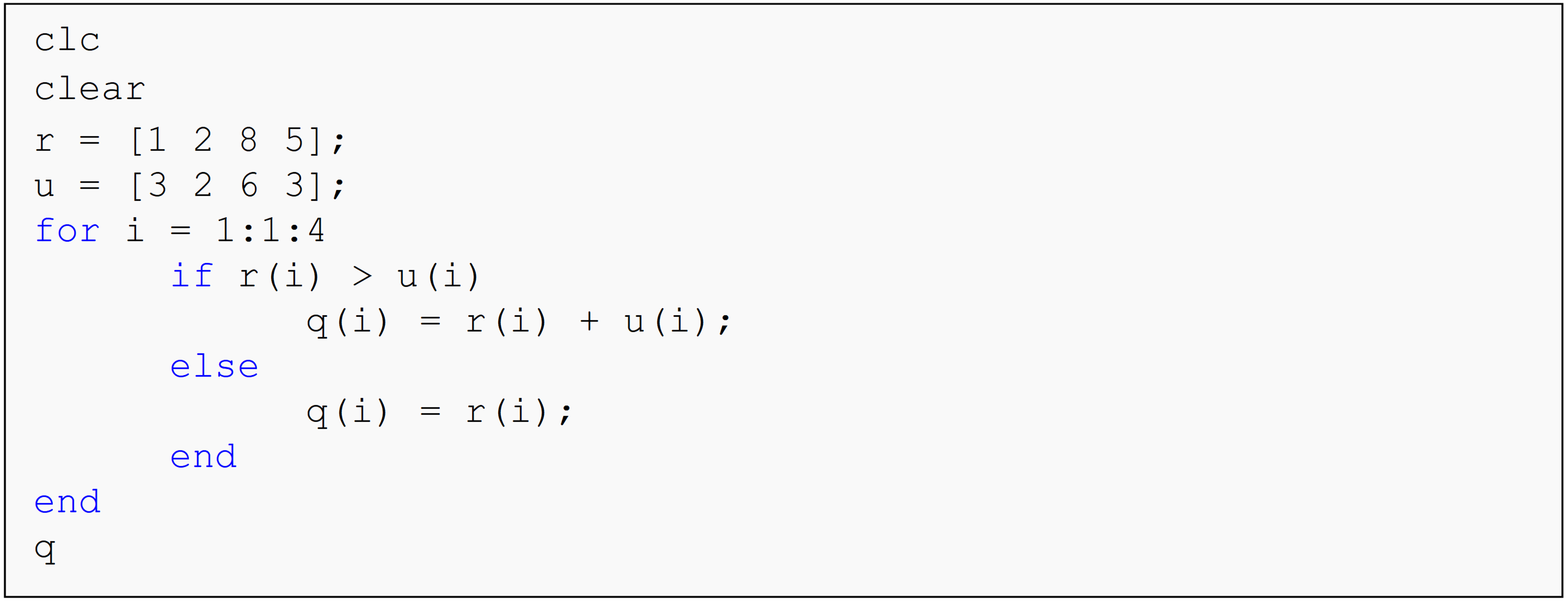
(a) q = [1 4 14 8]
(b) q = [1 2 8 5]
(c) q = [1 2 14 8]
(d) q = [4 2 6 3]
(3). The Command Window output of the following program is
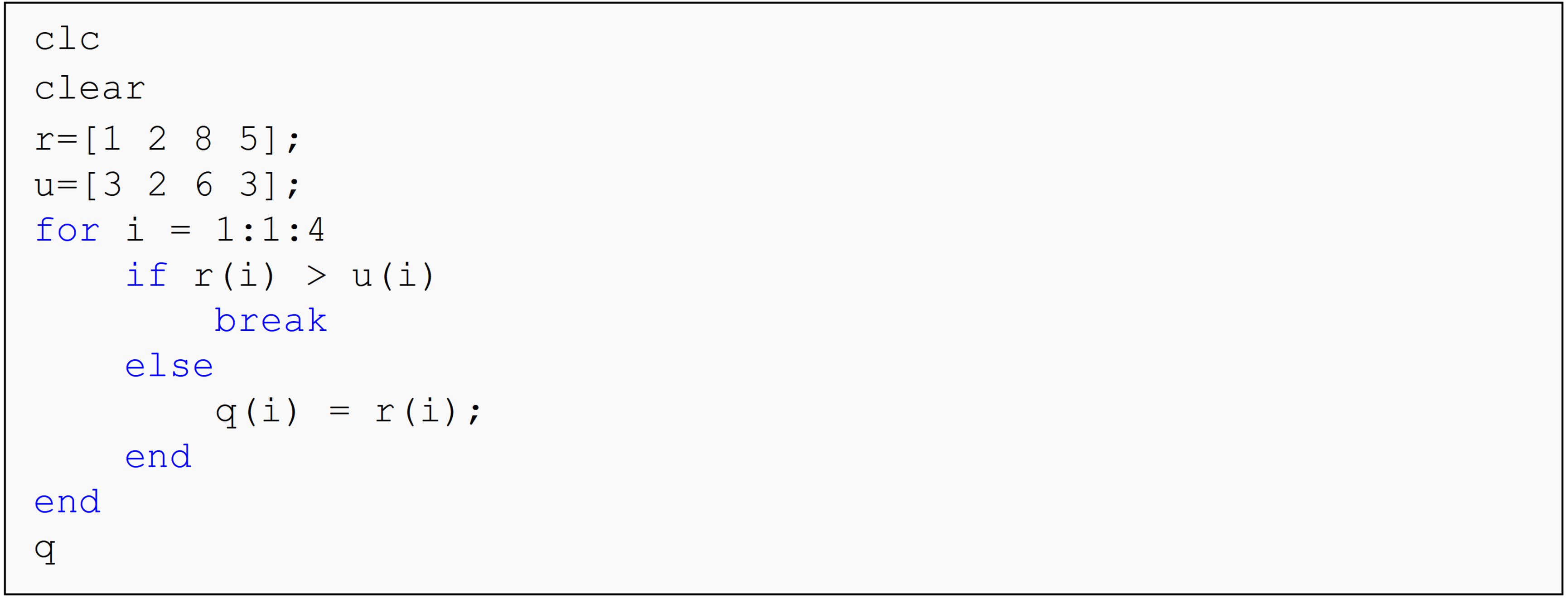
(a) q = [1 2]
(b) q = [3 2]
(c) q = [1 2 8 5]
(d) q = [3 2 6 3]
(4). The Command Window output of the following program is
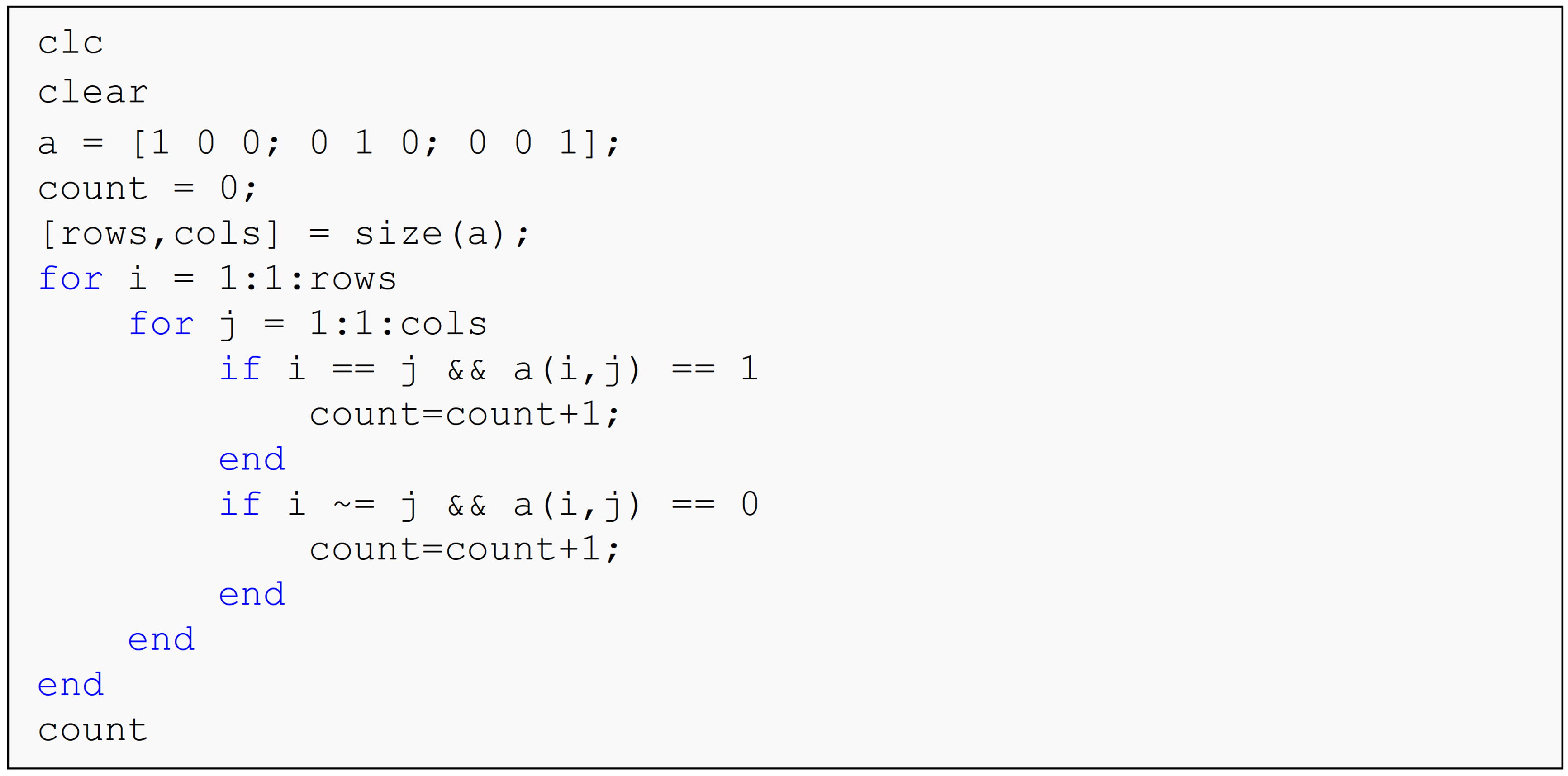
(a) count = 0
(b) count = 3
(c) count = 6
(d) count = 9
(5). The Command Window output of the following program is
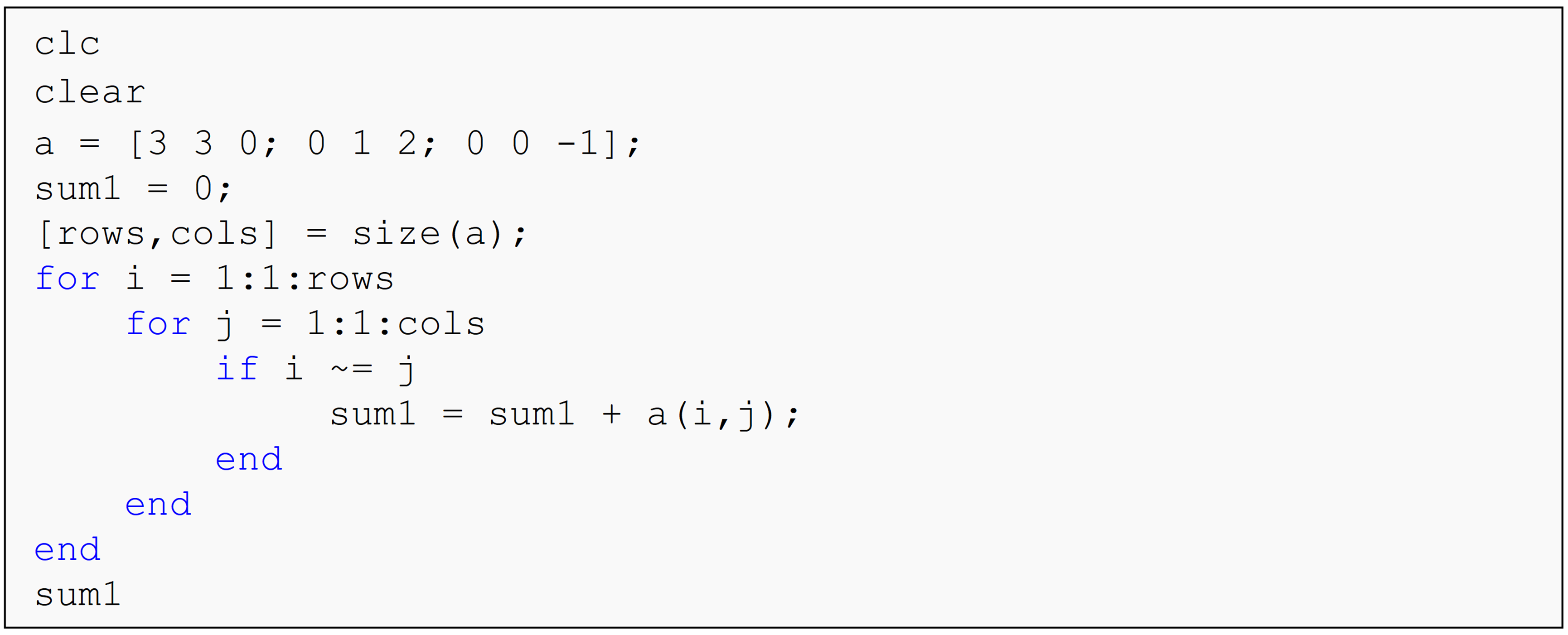
(a) sum1 = 2
(b) sum1 = 3
(c) sum1 = 5
(d) Undefined function or variable...
(6). The Command Window output of the following program is
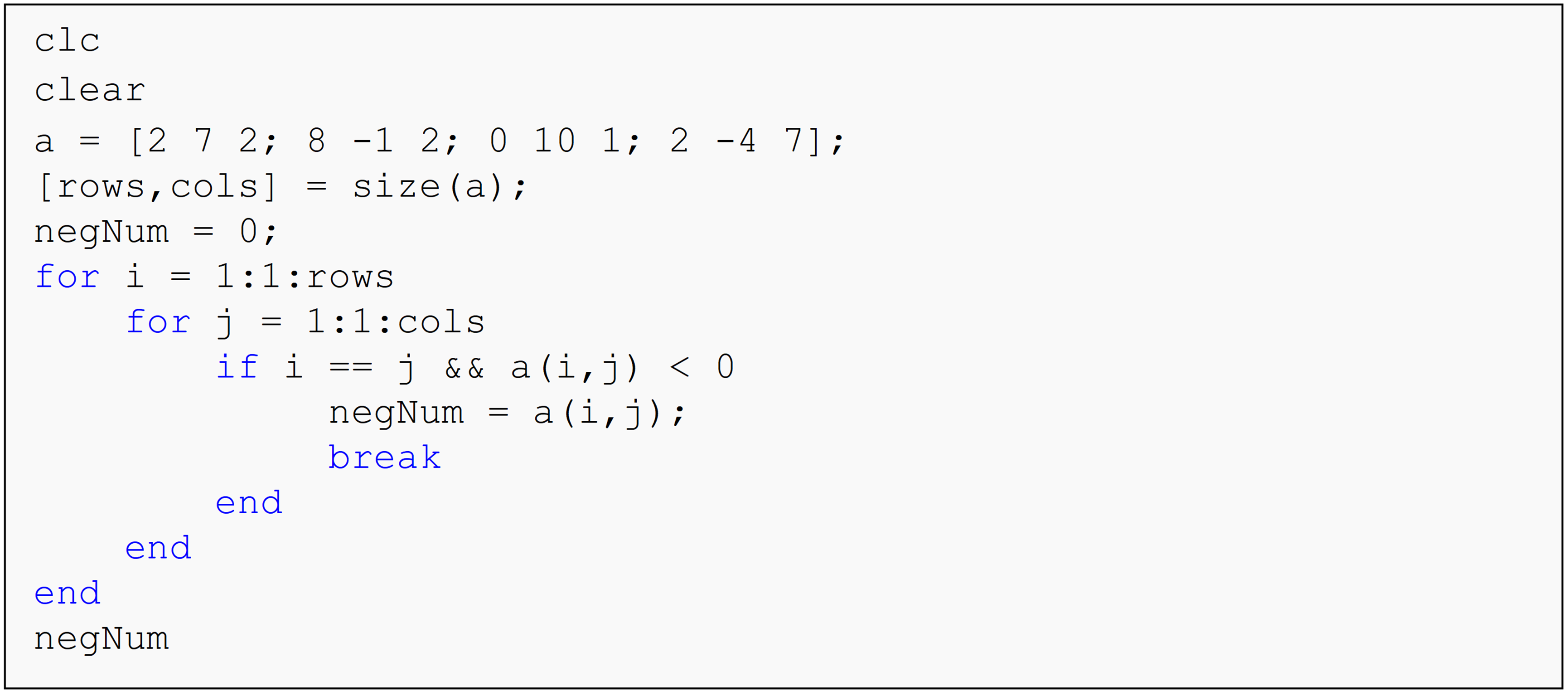
(a) negNum = 0
(b) negNum = -4
(c) negNum = -1
(d) Undefined function or variable...
Problem Set
(1). Using nested loops, write a program that outputs the sum, [A] + [B] of two equally sized matrices, [A] and [B]. Test and run your program for the following two matrices, [A] and [B].
\([A]=\begin{bmatrix} 0 & 5 & -3\\ 1 & -7 & 9\\ 5 & 5 & 12 \end{bmatrix}\) \([B]=\begin{bmatrix} 14 & 2 & 5\\ 1 & 7 & 3\\ 1 & 3 & 5 \end{bmatrix}\)
(2). Using nested loops, write a function that outputs the numeric value of the difference of two equally sized matrices, [A] and [B]. Test and run your program for the two following matrices, [A] and [B].
\([A]=\begin{bmatrix} 12 & 13 & 10\\ 7 & 9 & 13\\ 1 & 8 & 12 \end{bmatrix}\) \([B]=\begin{bmatrix} -14 & 10 & 5\\ -7 & 7 & 4\\ 2 & 0 & -9 \end{bmatrix}\)
(3). Write your own function, myDot, that finds the vector dot product of
two input vectors. The function inputs are two vectors, vec1 and
vec2, and the output is the value of the vector dot product. Do not
use the dot() or similar MATLAB functions.
Test your function for two vectors
vec1 = [3 -7 23]
vec2 = [-7 0 12]
(4). Without using the sum() function, write a function (myYoung) that
outputs Young’s modulus of a material based on an input of stress
vs. strain data. The stress and strain values must be entered using
two vectors, stress, and strain. The Young’s modulus (E), given
the stress (\(\sigma\)) and strain (\(\varepsilon\)) values, is found as
\[E = \frac{\displaystyle \sum_{i = 1}^{n}\sigma_{i}\varepsilon_{i}}{\displaystyle \sum_{i = 1}^{n}\left( \varepsilon_{i} \right)^{2}}\]
Test your function with the data provided in Table A.
Table A: Strain and Stress data of a material.
| Strain (m/m) | Stress (MPa) |
|---|---|
| 0.00010 | 19.10 |
| 0.00012 | 22.81 |
| 0.00100 | 187.0 |
| 0.00150 | 284.2 |
| 0.00180 | 344.3 |
| 0.00220 | 417.0 |
| 0.00260 | 495.0 |
(5). Write a program that determines if a square matrix, A is symmetric or not. A symmetric matrix is where \(a_{ij} = a_{ji}\) for all i, j. Matrix [A], given below, is an example of a symmetric matrix, which you can use to test your solution. The program needs to work for a square matrix of any size.
\[\left\lbrack {A} \right\rbrack = \ \begin{bmatrix} {2} & {8} & {9} \\ {8} & {4.5} & {6} \\ {9} & {6} & {-1} \\ \end{bmatrix}\]
(6). Write a program that outputs the value of the summation of the perimeter elements (outer elements) of a rectangular matrix. Use your knowledge of loops and/or conditional statements to write the program.
The program input is:
1) a rectangular matrix, rectMat.
The program output is:
1) the value of the summation of the perimeter elements, perimeterSum.
Test and run your program for the following \(3 \times 4\) matrix,
rectMat.
\[\begin{bmatrix}
2 & - 3 & 1 & 0 \\
5 & 7 & 1 & - 4 \\
9 & - 6 & 0 & 2 \\
\end{bmatrix}\]
Hint: The summation of the perimeter values for the above matrix is,
\(2 + ( - 3) + 1 + 0 + ( - 4) + 2 + 0 + ( - 6) + 9 + 5 = 6\).
(7). The column sum norm of a rectangular matrix [A] with m rows and n columns is defined as
\[norm\lbrack A\rbrack = \max_{1\leq j\leq n} \sum_{i = 1}^m|a_{ij}|\]
In other words, find the sum of the absolute value of the m elements
of each of the n columns. Then find the maximum of these n values
(do not use max(), min() or similar MATLAB function). This maximum
value is the norm of the matrix [A]. Using your knowledge of loops
and/or conditional statements, write the program that finds the norm
of an input matrix. Do not use norm() and other similar MATLAB
functions.
The program input is:
1) a rectangular matrix, mat.
The program output is:
1) the norm of the matrix, normMat.
Test and run your program with the following matrix, mat.
\[\begin{bmatrix} 25 & 20 & 3 & 2 \\ 5 & - 10 & 15 & - 25 \\ 6 & 16 & - 7 & 27 \\ \end{bmatrix}\]
Hint: Consider the following \(2 \times 3\) matrix, A
\[\lbrack A\rbrack = \begin{bmatrix} 6 & 3 & - 4 \\ 2 & 7 & 1 \\ \end{bmatrix}.\]
the norm[A] is found as follows:
Add absolute values of elements of first column, that is,
\(\left| {6} \right| + \left| {2} \right| = {8}\).
Add absolute values of elements of second column, that is,
\(\left| {3} \right| + \left| {7} \right| = {10}\).
Add absolute values of elements of third column, that is,
\(\left| - {4} \right| + \left| {1} \right| = {5}\).
The maximum then of the first, second and third column sum values is
maximum of \((8,\ 10,\ 5) = 10\). The norm of matrix [A], hence, is 10.
(8). A square matrix is considered bisymmetric if it is symmetric about both of its main diagonals. For example, consider the following \(5 \times 5\)matrix:
\[\begin{bmatrix} D_{1} & b & c & d & A_{1} \\ b & D_{2} & e & A_{2} & d \\ c & e & D_{3} & e & c \\ d & A_{2} & e & D_{2} & b \\ A_{1} & d & c & b & D_{1} \\ \end{bmatrix}\]
This matrix is symmetric about both main diagonals D and A, and therefore considered bisymmetric. Use your knowledge of programming concepts (loops and conditional statements) to write a program that outputs whether a square matrix is bisymmetric or not.
The program input is:
1) a square matrix, mat.
The program output is:
1) “Bisymmetric matrix” or “Not a bisymmetric matrix”
Test and run your program for the two matrices given on the next page.
\[\begin{bmatrix} 1 & 2 & 3 & 4 & 5 \\ 2 & 6 & 7 & 8 & 4 \\ 3 & 7 & 9 & 7 & 3 \\ 4 & 8 & 7 & 6 & 2 \\ 5 & 4 & 3 & 2 & 1 \\ \end{bmatrix} and \begin{bmatrix} 3 & 3 & 2 & - 1 \\ 3 & 4 & 6 & 0 \\ 2 & 6 & 4 & 3 \\ - 1 & 0 & 3 & 7 \\ \end{bmatrix}\]
(9). Using loops, write a program that transposes an input row vector. Do
not use the transpose() or equivalent function. The transpose of a
row vector is a column vector. For example
\[\begin{bmatrix} 1 & 2 & 3 & 4 \\ \end{bmatrix}^{T} = \begin{bmatrix} 1 \\ 2 \\ 3 \\ 4 \\ \end{bmatrix}\].
Test your program with the following vector.
a = [6 -6 4 13 0 7 2]
(10). Two matrices [A] and [B] can be multiplied only if the number of columns of [A] is equal to the number of rows of [B]. If [A] is a \(m \times p\) matrix and [B] is a \(p \times n\) matrix, then the resulting matrix [C] is a \(m \times n\) matrix. So how does one calculate the elements of [C] matrix?
\[c_{ij} = \sum_{k = 1}^{p}{a_{ik}b_{kj}} = a_{i1}b_{1j} + a_{i2}b_{2j} + \ldots\ldots + a_{ip}b_{pj}\]
for each \(i = 1,\ 2,\ldots\ldots,\ m,\text{and}j = 1,\ 2,\ldots\ldots,\ n\).
To put it in simpler terms, the ith row and jth column element of the [C] matrix in [C] = [A][B] is calculated as multiplying the ith row of [A] by the jth column of [B], that is,
\[\begin{split} c_{ij} &= \begin{bmatrix} a_{i1} & a_{i2} & \cdots & \cdots & a_{ip} \end{bmatrix} \begin{bmatrix} b_{1j}\\ b_{2j}\\ \vdots \\ \vdots \\ b_{pj}\end{bmatrix}\\ &= a_{i1}\ b_{1j}\ + \ \ a_{i2}\ b_{2j} + \ \cdots\cdots + \ a_{ip\ }b_{pj}.\\ &=\displaystyle\sum_{k=1}^pa_{ik}b_{kj} \end{split}\]
Complete the following:
(a). Write a function, myMult, that outputs the result of the multiplication of two matrices. The inputs are
first matrix,
[A],second matrix,
[B].
The output is
- the matrix
[C], where[C] = [A][B]
If the matrices cannot be multiplied, the output needs to be:
The matrices cannot be multiplied.
(b). Conduct the following tests of the function myMult in a testing
m-file
- Given
\[\lbrack A\rbrack = \begin{bmatrix} 5 & 2 & 3 \\ 1 & 2 & 7 \\ \end{bmatrix},\]
\[\lbrack B\rbrack = \begin{bmatrix} 3 & - 2 \\ 5 & - 8 \\ 9 & - 10 \\ \end{bmatrix},\]
find
\[\lbrack C\rbrack = \lbrack A\rbrack\lbrack B\rbrack\]
- Conduct two more appropriate tests of the function.